Magnetic Field Strength Based on Moving Point Charge
Magnetic field of a point charge + example of magnetic force between two charges – Zak’s Lab
First thing you want to do is recall the basics of what a vector is and what a cross product is.
- A vector has magnitude (size) and direction.
- A bar above a symbol (or sometimes the symbol bolded, or both) indicates that it’s a vector.
- Unit vectors are dimensionless vectors of magnitude 1 unit.
- For any given vector V̄ , its unit vector = V̄/|V̄|, where |V̄| is the magnitude of vector V̄
- Magnitude of cross product of vectors ā and b̄ is = |ā x b̄| = |ā||b̄|sin(θ)
- The result of ā x b̄ is another vector that is perpendicular to vectors ā and b̄
Assume we have a charge q moving at velocity v as shown in the drawing below.
Picture: B Located at Some Point , a Distance r from a Moving Charge q.
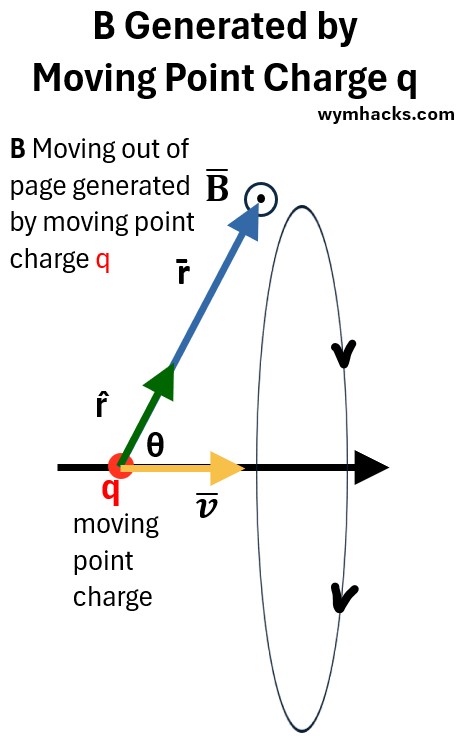
We can draw a position vector r̄ from q to the location at which we are measuring B.
- Let’s add a unit vector r̂ on the r̄ vector line as well.
The relationship of the magnetic field B̄ to a moving point charge q was determined experimentally (it was not derived from first principles).
It was constructed based on the following proportionalities.
The first two state that the magnetic field is proportional to the charge q and the speed v̄ of the charge.
1. B̄ ∝ q
2. B̄ ∝ v̄
We know that B is 0 when aligned with the v axis and maximum when perpendicular ( ⊥) to the v axis, so,
3. B̄ ∝ sin θ
Assume r̂ (r hat) is along the r̄ vector and is a unit vector (has magnitude 1), then we can state
4. B̄ ∝ (v̄xr̂ ) ∝ |v̄||r̂|sin θ ∝ |v̄||1|sin
Finally, the magnitude of B drops with increasing r similar to electric fields and gravitational fields.
5. B̄ ∝ 1/r2
Combine the above we get
the general formula for a field generated by a moving point charge (when v << speed of light).
B̄ = [μ0/(4π)]q(v̄xr̂)/r2
the magnitude of B is then [μ0/(4π)]q|v̄||r̂|sinθ)/r2 and |r̂| = 1 ; so, the magnitude of the Magnetic Field B is
B = [μ0/(4π)]qvsinθ/r2
where
- q = moving electric point charge
- v is the velocity of the point charge q
- B is the magnetic field
- μ0 = the permeability of free space or the magnetic constant.
- μ0 is a fundamental physical constant which shows how easily a magnetic field can pass through a vacuum
- μ0 = 4π×10−7 Tesla-meters/Amp = Henry/meters
- θ = angle between v̄ (v bar) and r̂ (r hat)
- r = distance from q to the point at which B is being measured
Current I in Terms of Drift Velocity
We are going to need to know the relationship between current I and drift velocity vd to derive the Biot-Savart equation.
First, what is drift velocity?
According to Wiki, “drift velocity is the average velocity that charged particles, such as electrons, attain in a material when an electric field is applied.
- Although individual electrons move randomly at very high speeds, the electric field causes a slight, net movement or “drift” in a specific direction.”
Consider a conductor with electrons flowing in the direction shown.
Picture: Electron Flow in a Conductor
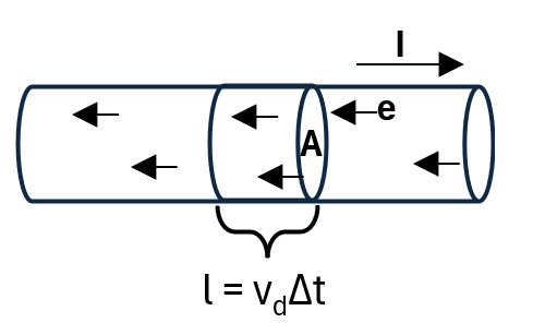
Let
1. n = the number of electrons per unit volume = #electrons/V
so,
2. N = number of electrons = nV where V is a volume we trace out after time Δt (starting at A).
Let
3. V = Al = AvdΔt
Substitute 3. into 2:
4. N = nAvdΔt
The total charge will therefore be
5. ΔQ = (N)(charge per electron) = (N)(e)
Substitute 4. into 5. to get
6. ΔQ = (nAvdΔt)(e)
Divide both sides by Δt
7. ΔQ/Δt = I = Current = neAvd
ΔQ/Δt = I = Current = neAvd ; I in terms of vd
Ok, we’ll use this in the next section.
Biot-Savart Law Derivation
Now, lets consider a very similar set up to B generated by a moving point charge i.e. B generated by a current.
Picture: B Generated by Current I Straight Wire
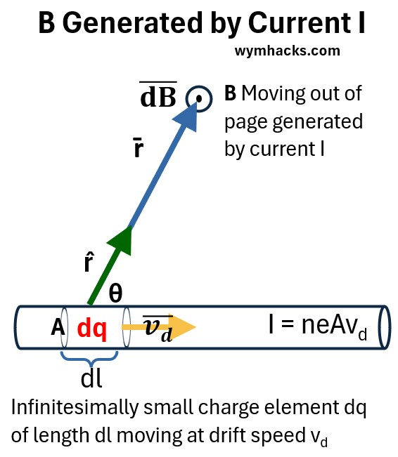
In this case we consider an infinitesimal length dl with an infinitesimal charge dq moving at a drift velocity v̄d.
And this causes an infinitesimal magnetic field dB̄ at a specific location r̄ away from the element.
Lets start with the general formula for a field generated by a moving point charge (when v << speed of light).
1. B̄ = [μ0/(4π)]q(v̄xr̂)/r2
Lets modify this to make it compatible with the way we defined the magnetic field, the charge , and the velocity.
2. dB̄ = [μ0/(4π)]dq(v̄dxr̂)/r2
We can express dq as follows (# charges/volume)(volume)(charge per charge carrier) =
3. dq = neAdl
- n = # charges per volume
- e = charge of an electron
- Adl = volume of charge element
substitute 3. into 2.
4. dB̄ = [μ0/(4π)]neAdl(v̄dxr̂)/r2
Let dl take the direction of v̄d
and move the magnitude of v̄d out in front
5. dB̄ = [μ0/(4π)]neAvd(dl̄xr̂)/r2
In the previous section we derived an expression for I in terms of the drift velocity
6. ΔQ/Δt = I = Current = neA vd
Substitute 6 into 5
7. dB̄ = [μ0/(4π)](I)(dl̄xr̂)/r2
dB̄ = [μ0/(4π)] (I) (dl̄xr̂)/r2 ; Differential Form of Biot-Savart Law
B̄ = [μ0/(4π)] (I) ∫ [ (dl̄xr̂)/r2 ] ; Integral Form of Biot-Savart Law
The magnitude of the vector dB̄ is dB and we know how to express it:
dB = [μ0/(4π)] (I) dlsinθ/r2 ; Magnitude of the Differential Form of Biot-Savart Law
where
- dB is the magnitude of an infinitesimally small magnetic field caused by infinitesimally small charge (current) element
- the vectors become scalars
- dl̄xr̂ = |dl̄||r̂|sinθ where | | is the magnitude symbol (by definition: see Vector Math)
- |r̂| = 1 (it’s a unit vector)
Recall the equation for the strength of an electric field caused by a point charge
E = kq/r2 ; E = strength of the electric field; k = Coulomb’s constant, q = magnitude of source charge, r = distance of E from point charge
It is structurally similar to the dB magnitude equation except for one huge difference: sinθ
For E, at a certain distance from r (anywhere) from the source charge, it is the same value.
But for dB, the strength will vary at the same r depending on the measurement point’s position relative to the charge (current) element.
- When perpendicular, dB will be maximum
- When parallel to the current element, it will be zero
Direction of B
There are two ways to determine the direction of the magnetic field B using the right hand.
- Put your thumb in the direction of current. Curling fingers are the direction of B
- Put back of palm on dl and sweep with fingers from dl̄ to r̂. Thumb points in direction of B.
Applying Biot-Savart to a Long Straight Wire
- The Derivative
- Geometry and Trigonometry Rules
- Integration Definition and Rules
- Derivation of the Biot-Savart law and calculating the magnetic field of a long straight wire – Zak’s Lab
Consider a long straight sire with current a perpendicular distance s away from a magnetic field B.
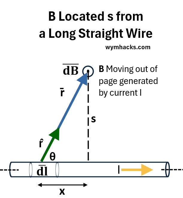
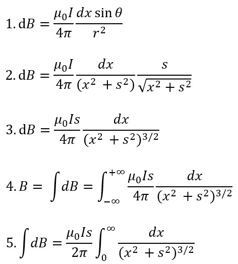
Starting with the Biot-Savart equation,
- substitute for r and sinθ using the triangle shape in the drawing above and the Pythagorean Theorem.
- r2 = (x2+s2)
- sinθ = s/r = s/√(x2+s2)
- simplify the (x2+s2) expression
- take the integral to find the magnitude B
- integrate over half the interval and then we’ll double the result at the end
- so bounds will now be from x=0 to ∞
Now,
- Let x = (s)tanθ
- so dx = (s)sec2θdθ
- See my post The Derivative for info on trig differentials
- Substitute x and dx into equation 5; (eqn. 6 )
- Simplify by taking s out of the integral; (eqn. 7 – 8)
- Substitute for the trigonometric identity (tan2θ + 1 = sec2θ); (eqn. 9)
- Simply the resultant sec2θ variables. ; (eqn. 10 – 11)
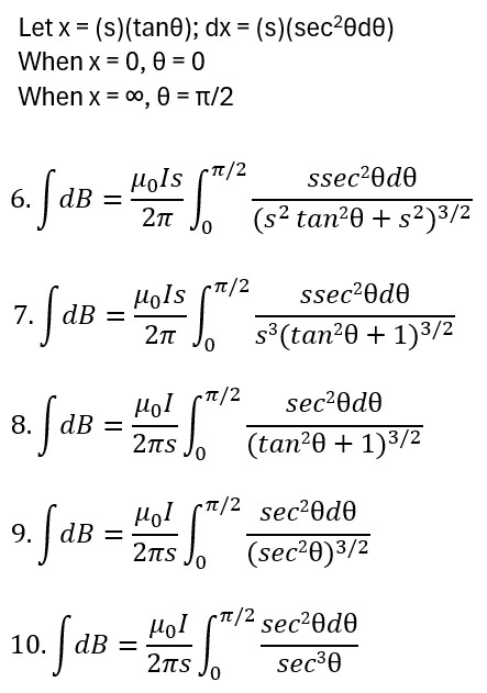
- Substitute cosθ for 1/secθ and take the integral of cosθ; (eqn. 12-14)
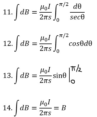
∫dB = B = μ0I/(2πs) ; B Near a Long Straight Wire with Current
Where
B = the magnitude of the magnetic field at a specific point.
- It is a vector quantity, so it also has a direction, which can be found using the right-hand rule.
- The SI unit is the Tesla (T).
I = The magnitude of the electric current flowing through the wire.
- The SI unit is the Ampere (A).
s = The perpendicular distance from the center of the wire to the point where B is measured.
- Note that s could be expressed as R or r or d etc.
- Just remember it’s the perpendicular distance to the wire.
- The SI unit is the meter (m).
μ0 = The permeability of free space, a fundamental physical constant.
- It represents how easily a magnetic field can be established in a vacuum. Its value is:
- μ0 =4π×10−7 AT⋅m
Magnetic Field (B) on a Closed Circular Loop Around A Wire with Current
This section is based on this great video by Zak’s lab: How to derive Ampere’s Law from the Biot-Savart Law: magnetic field due to enclosed current.
We want to derive the important Ampere’s Law and, we’re going to use the Biot-Savart equation to help us do this.
Consider a simple line current (shown in the picture below) which will of course generate a magnetic field.
- The I on the wire would be analogous to the enclosed point charges in Gauss’s Law for Electric Fields.
- A B field is generated which exists in a circular position around the wire.
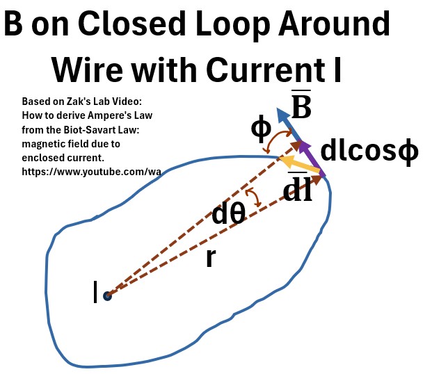
Picture: B on a Closed Circular Loop Around a Wire with Current I
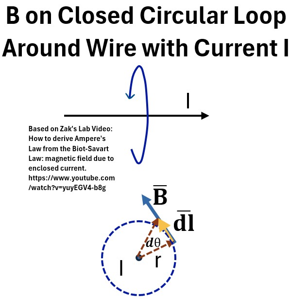
Let’s look at a plan view of the wire (the second picture above).
- The wire with current I is coming out of the page.
- B position of interest is r away from the wire on a closed loop around the wire
- This is due to the Right Hand Rule (RH thumb in direction of I, curled fingers then show B direction)
- A B̄ vector and a unit vector dl̄ parallel to it are shown.
- B̄ is tangential to the path.
An important distinction to be clear on as you read the following sections on Ampere’s Law:
- We are interested in a wire with current penetrating the imaginary surface a closed loop where the B field is.
Start with equation 14. from the last section.
- We are interested in a path integral in a loop around the wire carrying the current ∮B̄•dl̄
- Since B̄ and dl̄ are always parallel, ∮B̄•dl̄ can be expressed as just magnitudes
- B̄•dl̄ = Bdlcos(0) = Bdl (see Vector Math)
- We can also express dl as rdθ (see Geometry and Trigonometry Rules)
Substituting for B and dl, we get equation 15 (see below).
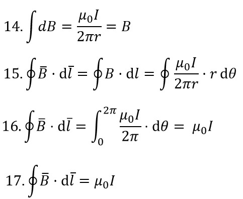
Simplifying equation 15 and integrating from 0 to 2π
gives equations 16 and 17.
This is Ampere’s Law which states:
The magnetic field circulating around a closed loop is directly proportional to the total electric current passing through (penetrating) that loop.
∮B̄•dl̄ = μ0I ; Ampere’s Law for A Circle Loop Enclosing A single Wire With Current I
To avoid confusion, sometimes the small l can be written as a capital L
∮B̄•dL̄ = μ0I ; Ampere’s Law for A Circle Loop Enclosing A single Wire With Current I
- ∮ is a closed line integral.
- i.e. summing up the contributions of the magnetic field along a complete, closed path, known as an Amperian loop.
- The integral path starts and ends at the same point.
- B̄ = Magnetic Field
- This is the magnetic field vector.
- B represents the magnitude and direction of the magnetic field at every point along the Amperian loop.
- Its SI unit is the tesla (T).
- dl̄ = dL̄ = Infinitesimal Line Element
- This is a small, infinitesimal vector segment of the closed loop.
- It points in the direction of the integration along the loop.
- Its SI unit is the meter (m).
- The dot product B̄⋅dl̄ calculates the component of the magnetic field that is parallel to the path element.
- μ0
= Permeability of Free Space.- A constant that represents the ability of a vacuum to support the formation of a magnetic field.
- Its value is approximately 4π×10 −7 T⋅m/A.
- I = Current:
- This is electric current that passes (penetrates) through the surface defined by the closed Amperian loop.
- It is a scalar quantity, and its SI unit is the ampere (A).
- Currents flowing in one direction are considered positive, and those flowing in the opposite direction are considered negative, according to the right-hand rule.
Magnetic Field (B) on a Closed Loop Around A Wire with Current
This section is based on this great video by Zak’s lab: How to derive Ampere’s Law from the Biot-Savart Law: magnetic field due to enclosed current.
Ampere’s law applies to any closed loop and not just a circular loop.
Consider the picture below which is very similar to the previous picture but for a non circular path.
Picture: B on a Closed Loop Around a Wire with Current
We want to take the line integral of the same expression again but lets simplify the B̄⋅dl̄ term first.
- Express B̄⋅dl̄ as BdlcosΦ
- Because this component is parallel to B, we can substitute rdθ for BdlcosΦ
- Substitute for B and BdlcosΦ and take the integral
- to get equation 19 which is the same as equation 17.
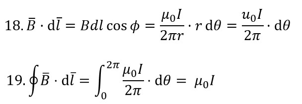
So Ampere’s Law doesn’t just apply to circles.
∮B̄•dl̄ = ∮B̄•dL̄ = μ0I ; Ampere’s Law for Any Loop Enclosing A single Wire With Current I
where
- ∮ is a closed line integral.
- i.e. summing up the contributions of the magnetic field along a complete, closed path, known as an Amperian loop.
- The integral path starts and ends at the same point.
B̄ = Magnetic Field
- This is the magnetic field vector.
- B represents the magnitude and direction of the magnetic field at every point along the Amperian loop.
- Its SI unit is the tesla (T).
dl̄ = dL̄ = Infinitesimal Line Element
- This is a small, infinitesimal vector segment of the closed loop.
- It points in the direction of the integration along the loop.
- Its SI unit is the meter (m).
- The dot product B̄⋅dl̄ calculates the component of the magnetic field that is parallel to the path element.
- μ0 = Permeability of Free Space.
- A constant that represents the ability of a vacuum to support the formation of a magnetic field.
- Its value is approximately 4π×10 −7 T⋅m/A.
- I = Current:
- This is electric current that passes through the surface defined by the closed Amperian loop.
- It is a scalar quantity, and its SI unit is the ampere (A).
- Currents flowing in one direction are considered positive, and those flowing in the opposite direction are considered negative, according to the right-hand rule.
Magnetic Field (B) on a Closed Loop Around Multiple Wires with Current
This section is based on this great video by Zak’s lab: How to derive Ampere’s Law from the Biot-Savart Law: magnetic field due to enclosed current.
Ampere’s law also applies when there are multiple wires with multiple currents penetrating a surface made by the loop.
Picture: B on a Closed Loop Around Multiple Wires with Current
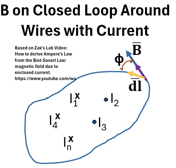
So we want to do the same path integral procedure, but this time we have to show each B produced by each I from each wire.
We can then express the path integral as shown in equation 20 below.
The dot product is distributive so, we can represent the equation as a sum of individual integrals for each B (equations 21 and 22) and we solve these the same way we did before.
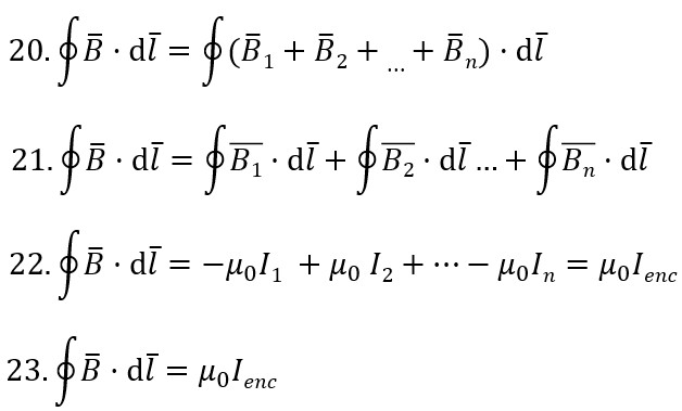
We have to give the proper sign for the components as shown in equation 22.
- For example: For current I1, I is going into the page, so by the Right Hand Rule, B is flowing clockwise
- We have to give it a negative sign because we set up the B in our drawing to flow counterclockwise.
- We do the same thing for the other Is
Ultimately we get to equation 23, Ampere’s Law again but now generalizing the current as the net (composite) current.
So, we can state Ampere’s law a little more generally as follows:
The Path integral of B̄⋅dl̄ on a closed curve is equal to μ0 times the net enclosed current passing through a surface defined by the curve.
∮B̄•dl̄ = ∮B̄•dL̄ = μ0Ienc ; Ampere’s Law for Any Loop Enclosing Multiple Wires With Current
where
- ∮ is a closed line integral.
- i.e. summing up the contributions of the magnetic field along a complete, closed path, known as an Amperian loop.
- The integral path starts and ends at the same point.
B̄ = Magnetic Field
- This is the magnetic field vector.
- B represents the magnitude and direction of the magnetic field at every point along the Amperian loop.
- Its SI unit is the tesla (T).
dl̄ = dL̄ = Infinitesimal Line Element
- This is a small, infinitesimal vector segment of the closed loop.
- It points in the direction of the integration along the loop.
- Its SI unit is the meter (m).
- The dot product B̄⋅dl̄ calculates the component of the magnetic field that is parallel to the path element.
- μ0 = Permeability of Free Space.
- A constant that represents the ability of a vacuum to support the formation of a magnetic field.
- Its value is approximately 4π×10 −7 T⋅m/A.
- Ienc = Enclosed Current:
- This is the net electric current that passes through the surface defined by the closed Amperian loop.
- It is a scalar quantity, and its SI unit is the ampere (A).
- Currents flowing in one direction are considered positive, and those flowing in the opposite direction are considered negative, according to the right-hand rule.
Magnetic Field (B) on a Closed Loop with A Wire (with Current) Not Penetrating Loop
This section is based on this great video by Zak’s lab: How to derive Ampere’s Law from the Biot-Savart Law: magnetic field due to enclosed current.
We need to show that: For a wire carrying a current that does not penetrate the “surface” of the loop, Ampere’s Law does not hold: ∮B̄•dl̄ = ∮B̄•dL̄ = 0
In the picture below, the wire is penetrating through the surface around which we are computing the B line integral.
This is a necessary condition to compute Ampere’s Law as we have done in previous sections.
Picture: Limits of Integration: B on Closed Loop with Wire Penetrating the Loop Surface
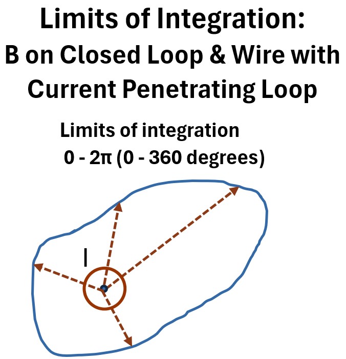
Notice that the integration limits we used to integrate Ampere’s Law were from 0 to 2π (the circumference of a circle).
But how would we define the limits for a wire that is not penetrating the loop.
See the picture below.
Picture: Limits of Integration: B on Closed Loop with Wire Not Penetrating the Loop Surface
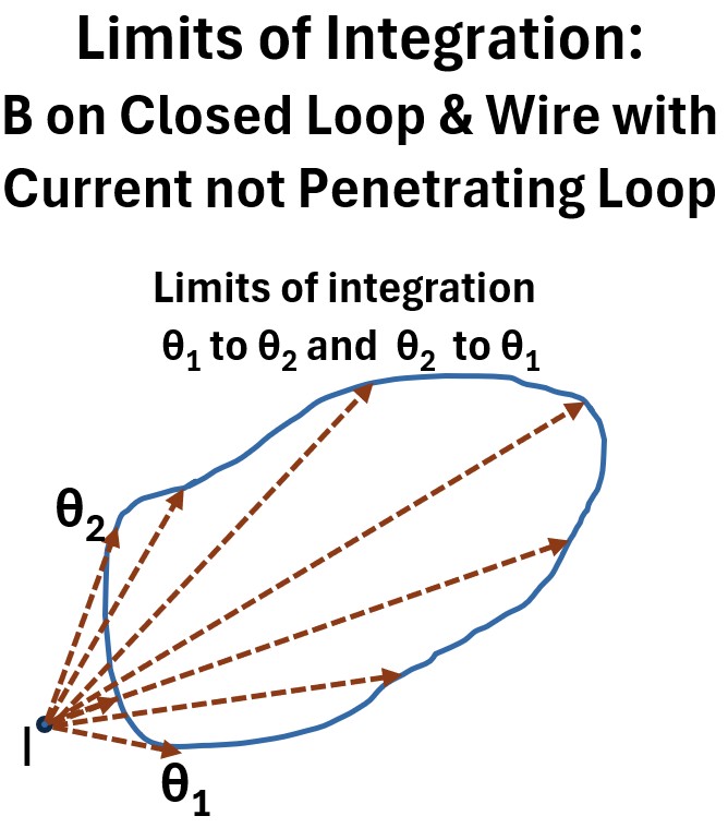
Now , the limits of integration as not going to go 360 degrees from 0 to 2π.
If we choose the lowest angle and the highest angle (θ1 and θ2) in the drawing above, the integration limits become
- θ1 and θ2 and
- θ2 and θ1
So lets do the line integral B̄⋅dl̄ again for a wire not penetrating the loop surface where we have to use these new limit ranges.
Picture: B on Closed Loop with Wire Penetrating Not Penetrating the Loop Surface
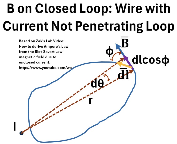
Starting with equation 18., we now have to do two integrals (eqn. 24) but for definite integrals, reversing the limits of integration changes the sign of the integral’s value (eqn. 25.)
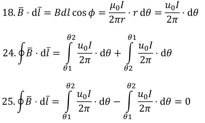
So, the integrals cancel out on the right hand side of equation 25 and we end up with a zero value.