SI Base and Derived Units (Quantities)
The International System of Units (SI) provides the standardized framework required for precise physical measurement and calculation.
This section defines the seven fundamental base units and demonstrates how they are mathematically combined to form derived units such as the Newton, Joule, and Watt.
These are essential for quantifying mechanical and electrical phenomena.
SI (International System of Units) defines seven base units which are
Time: second = s
Length: meter = m
Mass: kilogram = kg
Current: ampere = A = coulomb/s = C/s
Temperature: kelvin = K
Mole: mol
Candela: cd
I provide a few more details on Amperes and Temperature below.
You can review my post SI Base Units for more details.
You can also review some additional SI Related tabulations and charts in this post.
Regarding Amperes
The ampere is the unit of measure for electrical current.
- Current is the flow of electrons or charge.
- Flow of electricity along a wire conductor is current.
Its magnitude is set by fixing the numerical value of the elementary charge to be equal to exactly 1.602176634 x 10⁻¹⁹ coulombs (C)
Elementary Charge = 1.602176634 x 10⁻¹⁹ coulombs (C)
- The coulomb has SI units of As [ampere seconds],
Per NIST (adopted 2019), “The ampere is a measure of the amount of electric charge in motion per unit time ― that is, electric current.
But the quantity of electric charge by itself, whether in motion or not, is expressed by another SI unit, the coulomb (C).
One coulomb is equal to about 6.241 x 10¹⁸ electric charges (e).
One ampere is the current in which one coulomb of charge travels across a given point in 1 second.”
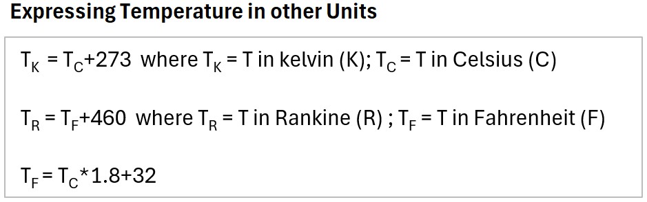
Regarding Temperature
- TK = TC +273 where TK = T in kelvin (K); TC = T in Celsius (C)
- TR = TF+460 where TR = T in Rankine (R) ; TF = T in Fahrenheit (F)
- TF = TC *1.8+32
Table: Expressing the SI Base Temperature in Other Units
Base Units
- Base Units are Independent Physical Quantities:
- They represent a distinct and independent physical quantity.
- They are irreducible dimensions of physical phenomena.
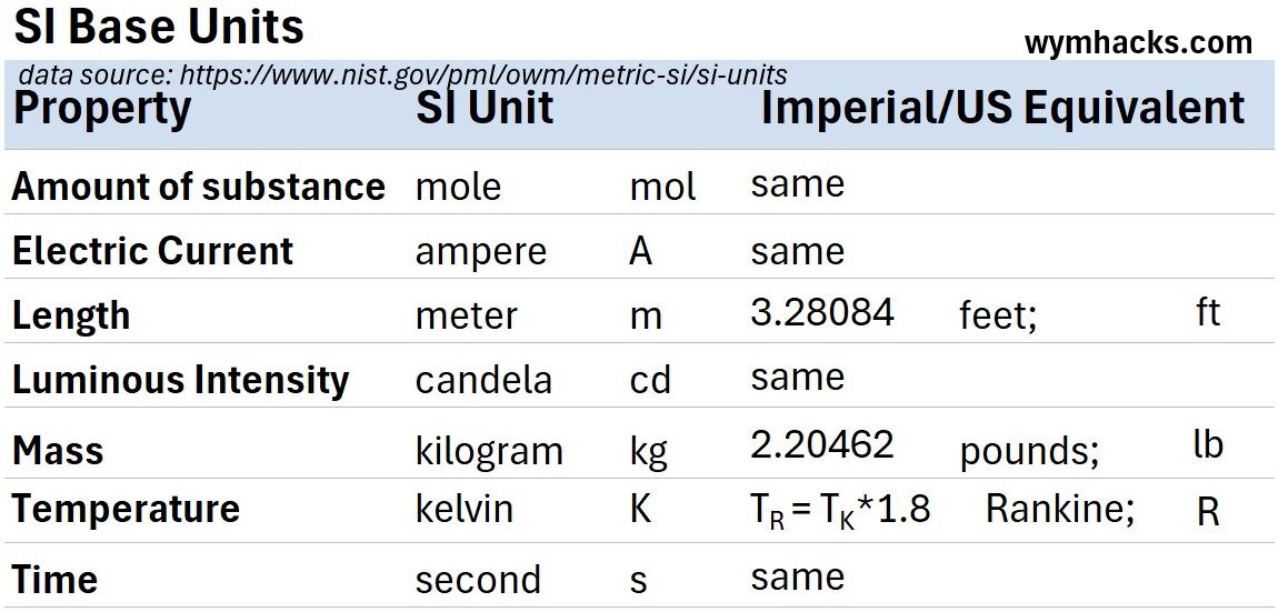
The table below shows the SI base units and the equivalent Imperial/US units.
Table: SI Base Units and Their Equivalent Imperial/US Units
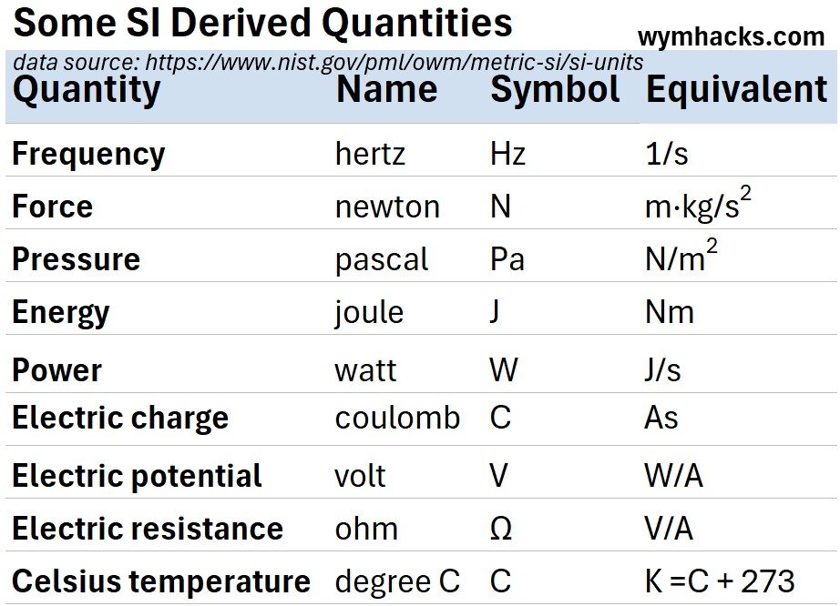
Derived Units
Table: SI Derived Quantities and Units
For a more complete tabulation of derived units you can check out my post: SI Base and Derived Units Tables and Charts
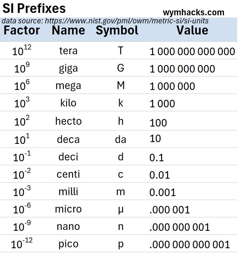
Numerical Prefixes
I list some metric SI prefixes in the table below.
For example, 1 picometer = 1×10-12 meters.
Table: Some Metric SI Prefixes
Vectors and Scalars
According to Google Gemini, “a vector is
- a mathematical object that possesses both a magnitude (a non-negative real number representing its “strength” or “length”) and
- a direction (an orientation in space).
It can be represented geometrically as a directed line segment (an arrow) where
- the length of the arrow indicates its magnitude, and
- the way the arrow points indicates its direction.”
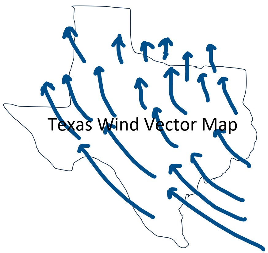
Have you seen those cool wind weather maps?
A lot of them display wind direction and magnitude with vector lines where shape and arrow show direction and the length indicates magnitude.
Picture: A Hypothetical Wind Vector Map for Texas
Some more examples of where vectors are used are:
Kinematics and Dynamics
- Describing motion (kinematics) and the causes of motion (dynamics) relies heavily on vectors.
- Displacement, velocity, and acceleration are all vector quantities.
- Forces are vectors; when multiple forces act on an object, vector addition (superposition) is used to find the net force and predict the object’s resulting motion.
- Without vectors, we couldn’t accurately model projectile motion, circular motion, or the complex interplay of forces in an engineered structure.
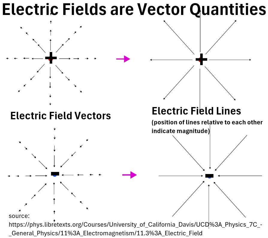
Electromagnetism
- Electric fields and magnetic fields are defined at every point in space with both a magnitude and a direction.
Picture: Electric Field Vectors and Lines
Picture: Magnetic Field Lines
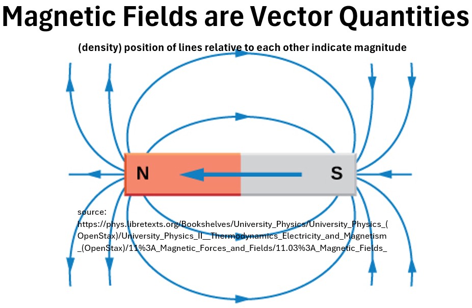
- Vector calculus, with operations like gradient, divergence, and curl, is indispensable for understanding how these fields originate from charges and currents, how they interact, and how electromagnetic waves propagate.
- Maxwell’s equations, which unify electricity and magnetism, are expressed most elegantly and powerfully in vector form.
Fluid Dynamics , Quantum Mechanics, etc.
Vector Basics: What is a Scalar?
A scalar only has magnitude (size).
Example: Speed as measured in meters/second.
Vector Basics: What is a Vector?
A vector has magnitude (size) and direction.
Example 1: Velocity has magnitude meters/second but also has a specified direction.
Example 2: Force has magnitude (measured in units of Newtons) and direction.
Vector Basics: Adding, Subtracting, and Multiplying Vectors
Check out my post on vector math to see how vectors can be added, subtracted, and multiplied (dot or cross).
Also check out these nice video tutorials on basic vector math:
Fields
This section is excerpted from my post on fields and field operators: Field Operators: Grad, Div, and Curl
In the sciences, a field represents a region of space where a physical quantity or mathematical value is assigned to each point.
- A field is a function that assigns a value (scalar or vector) to each point in a space.
- In physics, fields describe forces and influences extending through space and time, like gravity or electromagnetism.
Scalar Field (Scalar Field Function)
When the domain of a scalar function is a region in space (e.g., 2D or 3D physical space, or a surface), the scalar function effectively defines a scalar field.
A scalar field function is a type of scalar function that assigns a single scalar value to every point in a space,
Essentially, a scalar field is a specific application of a scalar function where the domain is a spatial region.
A generalized scalar field function, F, in three-dimensional space can be written as:
f(x,y,z)=C
where:
- x, y, and z are the coordinates of a point in space.
- C is a scalar value (a single number) assigned to that point.
For example, a scalar field could represent
- the temperature at every point in a room, where
- the function f(x,y,z) gives a single temperature value at a specific location.
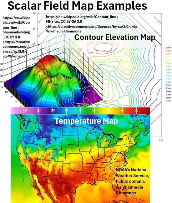
Other examples of Scalar Fields:
- Elevation contour map
- Pressure distribution
- Density (mass/volume) distribution

Vector Field (Vector Field Function)
A vector field function maps points in an n-dimensional space to vectors in that same n-dimensional space. e.g. 2D to 2D
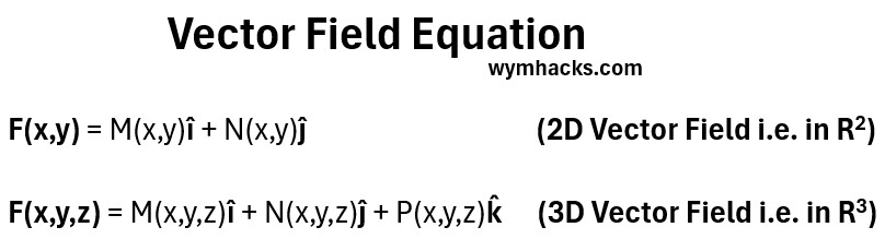
A generalized vector field function, F, in three-dimensional space can be written as:
F(x,y,z)=M(x,y,z)î + N(x,y,z)ĵ + P(x,y,z)k̂
where:
- x, y, and z are the coordinates of a point in space.
- î, ĵ , k̂ are the standard unit vectors along the x, y, and z axes.
- M, N, and P are scalar-valued functions that describe the components of the vector at each point.
For example, a vector field could represent the velocity of wind at every point over Texas,
- where M, N, and P would describe the x, y, and z components of the air’s velocity at that location.
In 2D, we would only have the x,y space and the î and ĵ unit vectors, and so the vector equation becomes:
F(x,y)=M(x,y)î + N(x,y)ĵ
That wind map of Texas shown in the previous section is an example of a vector field.
Vector Field Example: Wind Velocity and Direction Weather Map
Vector Field Example: Electric Field From A Single Positive Charge (Source: PHET)
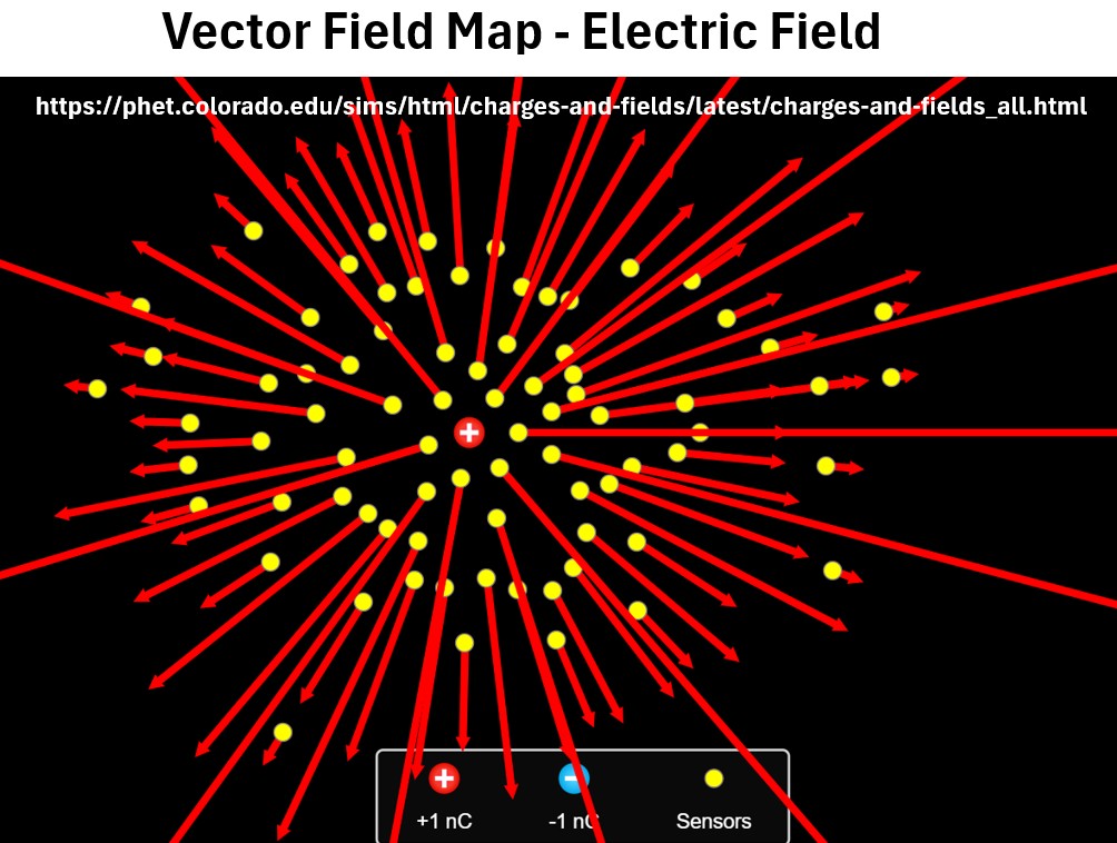
In the electric field map above, notice how the vectors all point out symmetrically and radially from the source charge.