Maxwell Equations – From Integral to Differential Forms

Introduction

Maxwell’s equations are typically first learned in their integral form, describing electromagnetism over volumes and loops.

However, to understand field behavior at specific points we must convert them into their differential form.

This post provides a technical walkthrough of that conversion.

We will apply the two primary links between vector calculus and physical space:

  • Gauss’s Divergence Theorem: To transform surface integrals into volume integrals.
  • Stokes’ Theorem: To transform line integrals into surface integrals.

By shifting from global boundaries to local derivatives, we arrive at the four partial differential equations that define modern classical electrodynamics

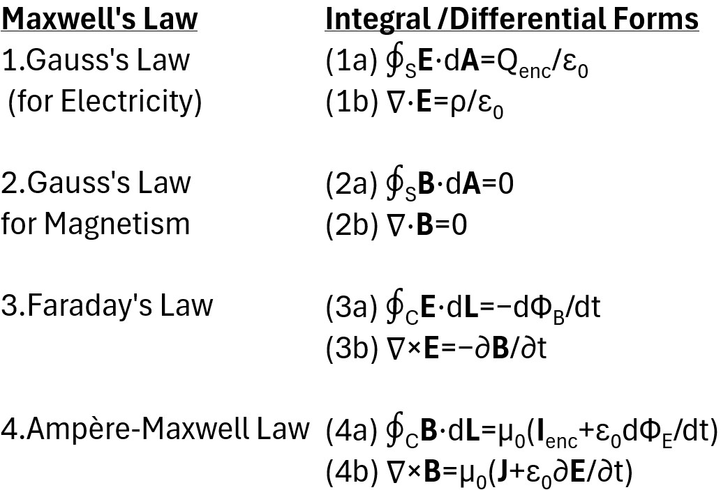
Table: Maxwell Equations Integral and Differential Forms

Return to Menu

Maxwell’s Equations – References

Return to Menu

Gauss’s Divergence Theorem and Stokes’s Theorem

We are going to use these two identities to convert Maxwell’s equations from their integral form to their differential form.

Gauss’s Divergence Theorem

The Divergence Theorem relates the flux of a vector field through a closed surface S to the divergence of the field over the volume V enclosed by that surface.

(1)  ∮sF̅•dĀ =∫v(∇•F̅)dV ; Divergence Theorem (Gauss)

See Appendix 1 for a simple explanation of the Divergence Theorem.

Stokes’s Theorem

Stokes’s Theorem relates the line integral of a vector field around a closed loop C to the integral of the curl of that field over the surface S bounded by the loop.
 
(2)  ∮cF̅•dL̅ =∫s(∇xF̅)•dĀ ; Stokes’s Theorem

See Appendix 2 for a simple explanation of Stokes’s Theorem.

Return to Menu

Gauss’s Law For Electric Fields: Integral to Differential Form

Let’s start with the Integral Form of Gauss’s Law for Electric Fields, one of the four Maxwell Equations

(1a) ∮sĒ•dĀ = qenclosed0 ; Gauss’s Law For Electric Fields ; Integral Form
  • Where q is the charge enclosed in the surface (any closed surface)
  • This equation is called Gauss’s Law for Electric Fields
  • It is the integral form of one of the four Maxwell Equations.
  • Ǖ = dot product of the electric field vector and the area vector.
  • ε= electric permittivity of free space
    • It is a fundamental physical constant that represents the ability of a vacuum to permit electric field lines.
    • ε0 = 8.854×10⁻¹² Farads per meter (F/m)

Let’s convert equation (1) to its differential form. 

Step (1): Charge Density Assumption: Assume the charge is distributed over the volume V with a density ρ .

(1.1) qenclosed  = ∫vρdV

Step (2): Substitute (1.1) into equation (1a)

(1.2) ∮sĒ•dĀ = ∫vρdV/ε= ∫vρ0dV

Step (3): Apply the Divergence Theorem: Replace the left hand side of (1.2) using equation (1) ∮sF̅•dĀ =∫v(∇⋅F̅)dV

(1.3) ∫v(∇⋅Ē)dV = ∫vρ0dV

Step (4): Localization: Since the volume V is arbitrary (it can be any size or shape), the only way for the integrals to always be equal is if the integrands are equal at every point:

(1b) (∇⋅Ē) = ρ0

The differential form of Gauss’s Law for Electric Fields clearly shows that the presence of charge density ρ  creates a “diverging” electric field.

(1b) ∇⋅Ē  = ρ/ε0 = 4πkρ ; Gauss’s Law for Electric Fields ; Differential Form

Variable Descriptions

  • ∮ = the surface integral over a closed surface
  • ∇⋅ = Divergence Operator where ∇ = nabla or del.
  • Ē = Electric Vector Field
  • ρ = charge density = charge/volume = q/V
  • ε= electric permittivity of free space
    • It is a fundamental physical constant that represents the ability of a vacuum to permit electric field lines.
    • ε0 = 8.854×10⁻¹² Farads per meter (F/m)
  • k = Coulomb’s Constant = electrostatic constant = 1/(4π ε0)  ≈8.99×10N⋅m2/C2
  • μ0 = magnetic permeability of free space = magnetic constant =  4π×10-7  H/m (Henrys per meter).
    • It is a fundamental physical constant that describes how a vacuum responds to a magnetic field.
  • c = 1/sqrt(μ0ε0) = speed of light = 299,792,458 m/s
  • π = pi = 3.1415..

Return to Menu

Gauss’s Law for Magnetic Fields: Integral to Differential Form

(2a) ∮s•dĀ = 0 ; Gauss’s Law for Magnetic Fields ; Integral Form
  • A closed surface integral of the dot product of B and A will equal zero.
  • The net magnetic flux through any closed surface is always zero.
  • It is the integral form of one of the four Maxwell Equations.
  • Magnetic monopoles do not exist.
  • Magnetic field lines never start or end at a point; they always form continuous, closed loops.
  • B = The Magnetic field (units: N/C)
  • B̄•Ā = dot product of the Magnetic field vector and the area vector. 

Step (1) Apply the Divergence Theorem: Replace the left hand side of (2a) using equation (1) ∮sF̅•dĀ =∫v(∇⋅F̅)dV
(2.1) ∫v(∇⋅B̄)dV = 0
 
Step (2) Localization: Since the volume V is arbitrary, the integrand must be zero everywhere:
(2b) (∇⋅B̄) = 0
 
(2b) (∇⋅B̄) = 0 ; Gauss’s Law for Magnetic Fields ; Differential Form

In magnetism, because the divergence is always zero, you can never have a source or a sink. This leads to two big real-world conclusions:

  • The Dipole Rule: Magnets always come in pairs (North and South).
    • If you snap a bar magnet in half, you don’t get a North piece and a South piece; you get two smaller magnets, each with its own North and South pole.
  • Continuous Loops: Magnetic field lines don’t start or stop anywhere; they form continuous, closed loops.
    • Every line that leaves the North pole must return to the South pole.

Return to Menu

Faraday’s Law: Integral to Differential Form

In this section we’ll use Stokes’s Law and the Leibniz Integration Rule to convert the integral form of Faraday’s Law into the Differential form.   

(3a) ∮Ē•dL̄ = −Nd/dt  ; Transformer EMF ; Faraday’s Law of Electromagnetic Induction (line integral form relating E to B)
  • This equation describes the phenomenon known as Transformer EMF (or non-motional ), where the electric field is induced by a time-varying magnetic field.

  • Name: It has different names
    • The Maxwell-Faraday Equation (Integral Form) – One of the four Maxwell Equations.
    • Faraday’s Law of Induction – Most common and general name
  • Physical Meaning:
    • The line integral of the induced electric field (E) around a stationary closed loop is equal to the negative rate of change of the magnetic flux () through the surface bounded by that loop.

  • Requirement:
    • The loop of integration (dL̄) must be stationary (fixed in space).
  • E is the electric field vector. It is an induced non conservative field (its not an electrostatic field).

    • We can express Eas E but just understand that it is induced.
  • dL̄ is the infinitesimal vector of a path element along a closed loop.
      • The direction of this vector is tangent to the path.
  • ∮ is a closed line integral. It means you are summing up the dot product of Ē and dL̄ along an entire closed loop.
      • The result of this integral is the electromotive force (EMF), which is the work done per unit charge in moving a charge around the closed loop.
      • For induced electric fields, this value is non-zero, indicating that the field is non-conservative.
  • N: # of coils
  • is the magnetic flux, which is a measure of the total number of magnetic field lines passing through a given surface
  • d/dt = Is the rate of change of magnetic flux with time
  • −: The negative sign represents Lenz’s Law.
    • It indicates that the direction of the induced electric field (and thus the induced current) will be such that it creates a magnetic field that opposes the change in the original magnetic flux.
    • This is a fundamental statement of energy conservation in electromagnetism.

We also know that 

(3.1) Φ = ∫sB̄•dĀ so let’s substitute this into the expression above to get

(3.2) ∮c•dL̄ = −Nd/dt = -Nd/dt∫sB̄•dĀ ; Transformer EMF ; Faraday’s Law of Electromagnetic Induction (line integral form relating E to B) 
Step (1) (Leibniz Integral Rule): Assume the surface S is stationary (not moving or changing shape).

This allows us to move the time derivative inside the integral as a partial derivative.

Assuming N=1, (3.2) becomes (see Appendix 3 for the details) :

(3.3) ∮c•dL̄ = s-∂B̄/∂t•dĀ

Step (2) Apply Stokes’s Theorem equation (2) ∮cF̅•dL̅ =∫s(∇xF̅)•dĀ  by converting the line integral on the left hand side of (3.3) into a surface integral of the curl.

(3.4) ∫s(∇xĒ)•dĀ = s-∂B̄/∂t•dĀ ; where I assume Ē = Ē

Step (3) (Localization): Because the surface S is arbitrary, the integrands must be identical and equation (3.4) becomes

 
(3b) ∇x = B̄/t ; Faraday Equation (Differential Form)

This shows that a changing magnetic field creates a “curling” electric field.

Return to Menu

Ampere-Maxwell Law: Integral to Differential Form

In this section we want to derive the differential form of the Ampere-Maxwell Equation.

(4a) ∮B̄•dL̄ = μ0Ienc + (μ0)(ε0)d/dt(sĒ•dĀ) ; Ampère-Maxwell Law

The Ampere-Maxwell Law states that the magnetic circulation around a loop is produced by two sources:

  • the enclosed current and
  • the time-varying electric flux (displacement current).

Variable descriptions are provided below.

  • ∮ is a closed line integral.
    • i.e. summing up the contributions of the magnetic field along a complete, closed path, known as an Amperian loop.
    • The integral path starts and ends at the same point.
  • B̄ = Magnetic Field
    • This is the magnetic field vector.
    • B represents the magnitude and direction of the magnetic field at every point along the Amperian loop.
    • Its SI unit is the tesla (T).
  • dL̄ = Infinitesimal Line Element
    • This is a small, infinitesimal vector segment of the closed loop.
    • It points in the direction of the integration along the loop.
    • Its SI unit is the meter (m).
  • The dot product B̄•dL̄ calculates the component of the magnetic field that is parallel to the path element.
  • ∮B̄•dL̄ ;  This term is called the circulation of the magnetic field.
  • μ= Permeability of Free Space.
    • A constant that represents the ability of a vacuum to support the formation of a magnetic field.
    • Its value is approximately 4π×10 −7 T⋅m/A.
  • ε0= 1/[4kπ]
  • ε0 = electric constant = electric permittivity of free space (i.e. a vacuum)
  • ε= 8.85 x 10⁻¹² C²/N⋅m² (or F/m).
  • Ienc = Enclosed Current:
    • This is the net electric current that passes through the surface defined by the closed Amperian loop.
    • It is a scalar quantity, and its SI unit is the ampere (A).
  • Φ= ∫Ē•dĀ = Electric Flux = a measure of the “flow” of an electric field through a given surface. 
  • Ē•dĀ = dot product of the electric field vector and the infinitesimal area vector. 
  • E/dt = is the rate of change of the electric flux over time

Assumptions

To perform this derivation, we make the following mathematical and physical assumptions:

  • Stationary Boundary: The contour C and surface sS are fixed in space (not moving or deforming).
    • This allows us to use the simplified Leibniz Integral Rule (see Appendix 3)
  • Continuity of Fields: B and E are well-behaved, continuous, and differentiable vector fields.
  • Current Density: The enclosed current  Ienc is the flux of a current density vector J through the surface S:

(4.1) Ienc = ∫sJ̅ •dĀ

Step (1): Use Stokes’ Theorem ((2)cF̅•dL̅ =∫s(∇xF̅)•dĀ) to convert the line integral of the magnetic field into a surface integral of its curl.

(4.2) ∮B̄•dL̄ = ∫s(∇xB̄)•dĀ) = μ0Ienc + (μ0)(ε0)d/dt(∫sĒ•dĀ)

Step (2): Apply Leibniz Rule to the Right Side Using the Leibniz Rule for a stationary surface, the total time derivative of the electric flux can be moved inside the integral as a partial derivative:

(4.3) ∮B̄•dL̄ = ∫s(∇xB̄)•dĀ) = μ0Ienc + (μ0)(ε0)(∫sĒ/∂t•dĀ)

Step (3): Substitute (4.1) into (4.3) and reorganize. 

(4.4) ∫s(∇xB̄)•dĀ) = μ0sJ̅ •dĀ + (μ0)(ε0)(∫sĒ/∂t•dĀ)

Move all the terms to the left hand side.

(4.5) ∫s(∇xB̄)•dĀ) –  μ0sJ̅ •dĀ –  (μ0)(ε0)(∫sĒ/∂t•dĀ) = 0

Group all terms under a single surface integral:

(4.6) ∫s( ∇xB̄ –  μ0J̅  –  μ0ε0Ē/∂t ) • dĀ = 0

Step (4): The Localization Argument. Since this integral must equal zero for any arbitrary surface S, the term inside the parentheses must be zero at every local point in space.

(4.7) = (4b) =  ∇xB̄ –  μ0J̅  –  μ0ε0Ē/∂t  = 0

Rearranging one last time we arrive at the differential form of the Ampère-Maxwell Law.

(4b) =  ∇xB̄ =  μ0 (J̅ + ε0Ē/∂t) ; Ampère-Maxwell Law; Differential Form

This equation shows that the “curl” (rotation) of the magnetic field at a point is caused by

  • the local Current Density J and
  • the local rate of change of the electric field: the term ε0Ē/∂t is called the Displacement Current. 

Return to Menu

Summary: Maxwell’s Equations

Table: Maxwell Equations

Maxwell Equations Integral and Differential Forms

1. Gauss’s Law for Electric fields
  • Integral Form:        ∮SE⋅dA=Qenc
  • Differential Form:  ∇⋅E=ρ/ε0
  • Meaning: Electric charges produce an electric field.
2. Gauss’s Law for Magnetic Fields 
  • Integral Form:        SB⋅dA=0
  • Differential Form:  ∇⋅B=0
  • Meaning: There are no magnetic monopoles; magnetic field lines are continuous loops.
3. Faraday’s Law
  • Integral Form:        CE⋅dL=−dΦB/dt
  • Differential Form:  ∇×E=−∂B/∂t
  • Meaning: A changing magnetic field induces an electromotive force (electric field).
 4. Ampère-Maxwell Law
  • Integral Form:         CB⋅dL0(Ienc0E/dt)
  • Differential Form:  ∇×B0(J0E/∂t)
  • Meaning: Magnetic fields are generated by moving charges (current) and changing electric fields.

Maxwell Equation Variables and Terms

  • E  / Electric Field / Volts per meter (V/m)
  • B  / Magnetic Flux Density (Magnetic Field) / Tesla (T)
  • ρ  /  Total Charge Density Coulombs per cubic meter (C/m³)
  • J  / Current Density / Amperes per square meter (A/m²)
    • J is the flow of actual electric charges (like electrons in a wire) per unit area
  • Qenc / Enclosed Electric Charge/Coulomb (C)
  • Ienc  / Enclosed Electric Current / Ampere (A)
  • Φ/ Electric Flux / V⋅m
  • ΦB / Magnetic Flux/Weber (Wb)
  • ε0E/∂t / Displacement Current /  Amperes per square meter (A/m²)
    • Displacement current isn’t actually “current” (moving charges); it’s a changing electric field that acts like a current by producing a magnetic field.
    • It’s Maxwell’s “mathematical glue” that ensures magnetic fields still exist in gaps—like between capacitor plates—where physical electrons aren’t flowing

Maxwell Equation Constants

  • ε/  Permittivity of Free Space/  8.854×10⁻¹² F/m
  • μ/  Permeability of Free Space/  4π×10−7 H/m
  • c  /  Speed of Light in Vacuum/  299,792,458 m/s (c=1/μ0ε0)

Maxwell’s Equations Operators

    • Del (Nabla)
    • Vector differential operator
    • Represents the rate of change in 3D space.
  • ∇⋅
    • Divergence
    • “Flux per unit volume”
    • Measures if a field is “spreading out” from a point (source) or “shrinking” into it (sink).
  • ∇×
    • Curl
    • “Rotation”
    • Measures the tendency of a field to circulate or “spin” around a point.
  • ∂/∂t
    • Partial Time Derivative
    • Temporal change
    • Measures how the field changes at a fixed point as time passes.
  • S
    • Surface Integral
    • Total flux through a surface
    • Sums the field components passing perpendicularly through a closed surface.
  • C
    • Line Integral
    • Circulation around a path
    • Sums the field components tangent to a closed loop.
  • dA
    • Differential Area
    • Vector Surface element
    • A vector normal (perpendicular) to the surface.
  • dL
    • Differential Path Vector
    • Path element
    • A tiny vector tangent to the integration loop.

Appendix 1: Divergence Theorem Explained

Think of the Divergence Theorem as a way of counting how much “stuff” is being created inside a container by just looking at how much “stuff” is leaking out of the walls.

Here is the breakdown of the intuition:

The Analogy: The Magic Room

Imagine you have a room full of people.

  • Flux (The Boundary): You stand outside the room and count how many people walk out the door minus how many walk in. If 10 people leave and only 2 enter, the “net flow” out of the room is +8.
  • Divergence (The Interior): You go inside the room and find out why that happened. You find a secret teleporter (a Source) that just beamed 8 new people into the room.
  • The Theorem: The Divergence Theorem simply says that if 8 people were created inside (Sum of Divergence), then 8 people must have crossed the boundary (Net Flux).

What “Divergence” Actually Means

Divergence measures how much a vector field “spreads out” from a single point.

  • Positive Divergence (+): A Source. Like a sprinkler head spraying water out.
  • Negative Divergence (-): A Sink. Like a drain sucking water in.
  • Zero Divergence (0): Like a steady river. Water flows in one side and out the other, but no water is being created or destroyed at that spot.

Why the Math Works

The math looks scary (1) ∮sF̅•dĀ =∫v(∇⋅F̅)dV, but the logic is simple:

  • Imagine a giant box. Inside that box are millions of tiny “mini-boxes.”
  • In every tiny box, if stuff flows out of its right side, it immediately flows into the left side of the box next to it.
  • Because they are touching, all the flow inside the giant box cancels out.
  • The only flow that doesn’t get canceled is the flow at the very edge—the outer walls of the giant box.
  • Therefore, adding up all the tiny “creations” (divergence) inside equals the total amount that “leaks” out of the big surface (flux).

How we used it for Maxwell

When we converted Gauss’s Law:

  • The Integral form said: “The total electricity leaking out of this bubble depends on the total charge inside.”
  • The Divergence Theorem let’s us express the differential form of Gauss’s Law  (5) ∇⋅Ē  = ρ/ε0 = 4πkρ
    • i.e. at every single point inside, the ‘spreadiness’ of the electric field (∇⋅Ē) is proportional to the charge density (ρ) at that point.”

It’s essentially moving from a “global” view (the whole bubble) to a “local” view (a single point).

Return to Menu

Appendix 2: Stokes’s Theorem Explained

If the Divergence Theorem is about “leaks” and “sources,” Stokes’s Theorem is about “whirlpools.”

The Analogy: The Paddle Wheel

Imagine you have a big tub of water and you draw a circle on the surface with a marker.

  • The Boundary (Line Integral): You walk around the edge of that circle and measure how fast the water is moving along the path with you. 
  • If the water is spinning fast, you’ll feel a lot of “push” as you walk the circle.
  • The Interior (Curl): Now, imagine you drop thousands of tiny little paddle wheels into the water inside that circle. 
  • If the water is “curling” (spinning) at any point, those little paddle wheels will start spinning in place.
  • The Theorem: Stokes’s Theorem says that if you add up the spin of all those tiny paddle wheels inside the circle, it will equal the total “push” you felt while walking around the edge.

What “Curl” Actually Means

In math, we write this as ∇ x F̅.

It measures the rotation of a field at a specific point.

  • High Curl: Like the center of a tornado or a whirlpool.
  • Zero Curl: Like a smooth, straight-moving highway.
    • Even if the cars are going fast, they aren’t turning, so a paddle wheel placed between lanes wouldn’t spin.

Why the Math Works (The “Cancellation” Trick)

Just like the Divergence Theorem, this works because of cancellation:

  • Imagine your big circle is actually made of two smaller squares side-by-side.
  • If the water is spinning clockwise in both squares, then in the middle—where the two squares touch—the water is moving UP for one square and DOWN for the other.
  • Those two middle movements cancel each other out.
  • The only movements that don’t get canceled are the ones on the very outside edge of the big shape.
  • So, the sum of all the “tiny spins” inside equals the “big spin” around the boundary.

How we used it for Faraday’s Law

When we converted Faraday’s Law:

  • The Integral form said: “If the magnetic flux through this loop changes, it creates a voltage (push) all the way around the wire loop.”
  • Stokes’s Theorem let’s us say: “Therefore, a changing magnetic field creates a ‘whirlpool’ of electric field ∇ x Ē at that exact point in space.”

Summary: The Two Big Tools

Divergence Theorem
  • Focus: Sources/Sinks
  • What it measures: Is stuff being “created” or “destroyed”?
  • Boundary: A Surface (like a balloon)
Stokes’s Theorem
  • Focus: Rotation/Twist
  • What it measures: Is the field “spinning” or “curling”?
  • Boundary: A Loop (like a rubber band)

Return to Menu

Appendix 3: Leibniz Rule

The General Leibniz Rule for Surfaces

We start with the integral form (for N=1) of Faraday’s Law. 

(A3.1) = (3b) = ∮c•dL̄ -d/dt∫sB̄•dĀ

Where C is a closed contour and S is the surface bounded by that contour.

To move the time derivative inside the surface integral, we invoke the Leibniz Integral Rule for a two-dimensional surface moving in three-dimensional space. The general rule is:

(A3.2) d/dt∫s(t)B̄•dĀ = ∫s(t)∂B̄/∂t•dĀ +∫s(t)(∇B̄)v̅•dĀ -∮s(t)(v̅xB̄)•dL̄

or

(A3.3) d/dt∫s(t)B̄•dĀ = s(t)(∂B̄/∂t + (∇B̄)v̅)•dĀ – s(t)(v̅xB̄)•dL̄

Specific Assumptions for Transformer EMF:

  • Stationary Loop: We assume the loop C and surface S are fixed in space and do not change shape over time. Therefore, the velocity of the boundary v̅ = 0.
  • Solenoidal Field: Since ∇B̄ = 0  (Gauss’s Law for Magnetic Fields), the divergence term vanishes regardless of motion.
(A3.4) d/dt∫s(t)B̄•dĀ = ∫s(t)∂B̄/∂t•dĀ 
(A3.5) = (3.2) = ∮c•dL̄ = s-∂B̄/∂t•dĀ

Assume E= E = E induced.

Return to Faraday Section

Disclaimer: The content of this article is intended for general informational and recreational purposes only and is not a substitute for  professional “advice”. We are not responsible for your decisions and actions. Refer to our Disclaimer Page.

Leave a Comment

Your email address will not be published. Required fields are marked *