Mortgage Basics
What is a mortgage?
According to the Consumer Financial Protection Bureau, a “mortgage is an agreement between you and a lender that gives the lender the right to take your property if you fail to repay the money you’ve borrowed plus interest.” So, a mortgage loan is secured by the property itself. What is a Home Mortgage then?
A home mortgage has to do with borrowing money for purchasing residential property.
Home Mortgages
A home mortgage is a type of annuity. I cover annuities in detail (including derivations) in my blog, “Time Value of Money (TVM) Concepts, Formulas and Functions”.
Annuities are constant (or constantly growing) and even (equal interval), periodic cash flows that occur (typically) weekly, monthly, quarterly, or yearly . They last for a finite period of time. Annuities are employed in all sorts of financial calculations (e.g. investments, retirement planning, mortgages and other loans, education cost planning, etc.).
Consider a simple example of three yearly cash flows occurring in the timeline shown in Schematic 2.1 Below. Schematic 2.1 defines various types of annuities in terms of timing of constant or growing cash flows.
Schematic 2.1 – Annuity Definitions on a 3 Year Timeline Example
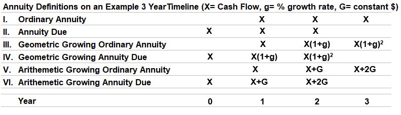
An Ordinary Annuity has constant cash flows occurring at the end of the period as shown in row I. of Schematic 2.1.
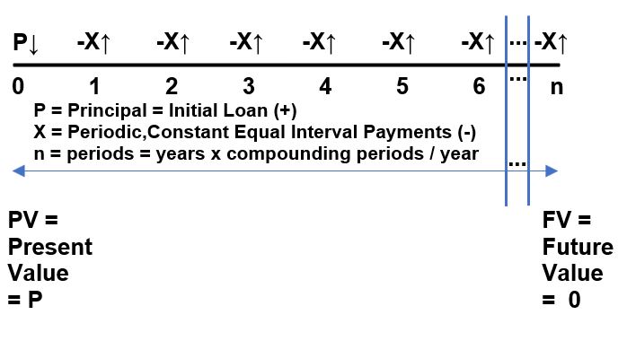
Fixed rate home mortgages are examples of Ordinary Annuities where a loan is provided (positive cash flow) and the borrower has to pay back the loan via equal and regular payments (negative cash flows) for the duration of the loan (at a fixed interest rate that is applied at a fixed frequency). Schematic 2.2 shows this generically in a timeline.
Schematic 2.2 – Generic Timeline for a Fixed Rate Home Loan (Ordinary Annuity)
The same process might be applied to other loans (e.g. car loan), but we’ll work through the concepts assuming we have a home loan.
- Cash flow direction must be defined as (+) for inflows of cash (e.g. the loan received P = PV) and (-) for cash outflows (e.g. the payments X).
- The PV or Present Value or Principal is the starting loan amount (the original loan). It’s a cash inflow, so it will have a positive sign convention.
- Given a fixed annual interest rate (i) applied at a fixed frequency (c) and the duration of the loan (y years), a constant payment X can be calculated. X is an outflow and so has a negative sign convention.
- For fixed rate home loans in the United States, the interest frequency (compounding frequency) is typically monthly (in Canada, it’s typically Semi-Annually).
- For monthly compounding periods, there are 12 payments (X) per year. (e.g. a 30 year loan will have c x y = n = 12 x 30 = 360 payments). The applied interest rate will be i/c = 7%/12 = .58333%.
- The FV of the loan, at the end of the loan duration, will be 0 (it’s when the loan is paid off so FV at time y = 0).
Amortization
Consider taking out a US home loan (P) for $500,000 that has a fixed annual interest rate of 7%, where payments are made monthly, and the duration of the loan is 30 years. Knowing these values allows the lender (and you) to compute a payment schedule that might look like the following Schematics 2.3a and 2.3b.
Schematic 2.3a – First Six Payments of a 30 year 500,000 loan at a fixed rate of 7%
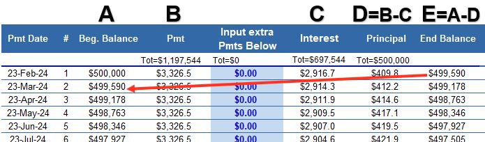
The table above shows the first 6 payments of the loan.
- In column B, a fixed payment of $3,326.5 is computed and entered into the first row (and every row). This is computed using the Present Value Ordinary Annuity (PVOA) equation which we’ll cover in the next section. It’s the exact amount needed to be paid each month for 30 x 12 = 360 months in order for the loan to be fully paid back. It is the X in Schematic 2.2.
- The Interest applied to the principal will be 7% applied monthly, so the monthly rate is 7%/12 = .58333…%.
- Multiplying the Beginning Balance in column A by the monthly interest rate will give the Interest portion of the payment in column C.
- The Principal portion of the payment is just the difference between the Payment and the Interest (the values in Columns B and C). So, Col. D = Col. B – Col. C.
- The Ending Balance is then the Beginning Balance minus the Principal portion of the payment (Col. E = Col A. – Col. D).
- This Ending Balance becomes the Beginning Balance for the next monthly payment.
- We do the same calculations in row 2, row 3,…, all the way down to row 360 to fully pay off the loan (assuming no extra payments are made).
Schematic 2.3b – Last Five Payments of a 30 year 500,000 loan at a fixed 7%
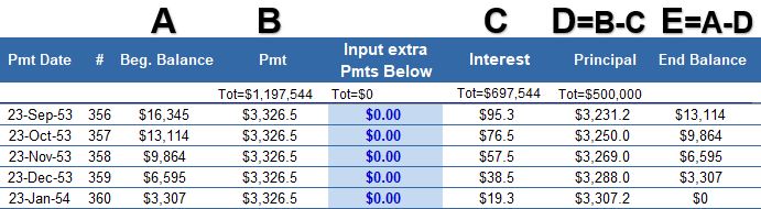
- With each progressive row, the interest portion of the payment decreases, and the principal portion of the payment increases.
- The balance (the remaining amount of the loan principal) goes to exactly zero with the last payment (the 360th payment)
This payment breakdown into an Interest portion and a Principal portion might seem odd, almost arbitrary. But, it’s not.
Look at Schematic 2.2 again. With each progressive payment, the amount owed is decreased by the Principal portion of the payment for that period. The subsequent Interest portion of the payment is based on this reduced outstanding balance. So the Interest and Principal portions of the payments are exactly correct and based on the exact total payment (of $3,326.5 in this example). Capiche?
This gradual payoff of the Principal (loan) is called amortization and its root comes from the Latin Admortire = to kill. Amortization is the gradual “killing” of the loan with each payment.
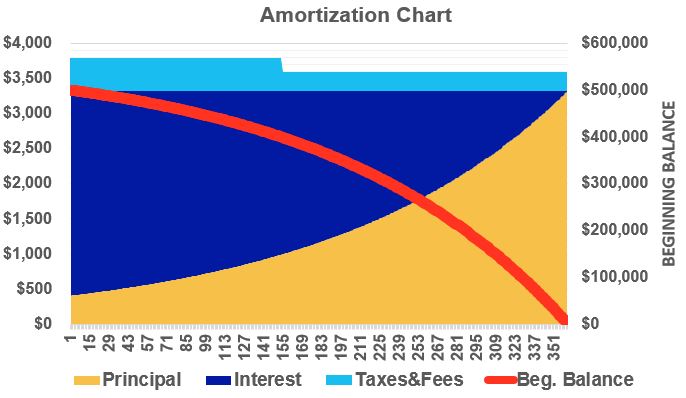
We can produce a cool looking graph (Schematic 2.3c below) showing the time progression of the monthly payments of principal, interest, taxes and fees (as area curves read off the left axis) and the remaining balance (the curved line that you read off of the right axis).
Taxes and fees are additional costs that are normally included in these charts. They can include monthly (or equivalent monthly) fees for property taxes, home insurance , and other fees. There will be one-time closing costs as well that don’t show up on these graphs but can be substantial. See Appendix 5 for more on typical home mortgage recurring (PITI – Principal, Interest, Taxes, Insurance) costs and one-time closing costs.
Schematic 2.3c – Amortization Chart for a 30 year, $500,000 lone at a fixed 7%
Next, let’s describe some of the key mortgage equations.
Mortgage Equations Derived from the PVOA
Schematic 3.1 below is the Generic Home Mortgage Timeline we showed earlier.
Schematic 3.1 (Schematic 2.2) – Generic Home Mortgage Timeline
This timeline setup can be described by the Present Value Ordinary Annuity (PVOA) equation. Refer to my blog, “Time Value of Money TVM Concepts Formulas and Functions“ for much more on PVOAs (and other annuity types) and how the equation is derived.
Equation 3.1 (Equation A1.1) – Present Value Ordinary Annuity (PVOA)
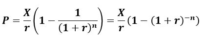
- P = principal (i.e. loan amount)
- X = constant and equal interval payments
- r = interest rate = i/c = (annual interest rate)/(number of compounding periods per year)
- n = number of compounding periods = (c)(y) where y = loan duration in years
The Present Value Ordinary Annuity (PVOA) equation can be used to solve
- for P, the present value (Principal or Loan).
- for X, the constant periodic payment.
- for the time duration y where n = (c)(y) = compounding periods/year “times” the number of years
These are listed below in their explicit forms. Please refer to Appendix 1 for more derivation details.
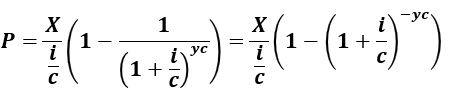
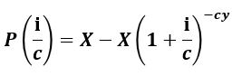
Mortgage Equation for P (Principal or Loan Amount)
Equation 3.2 (Equation A1.4):
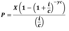
Use Equation 3.2 (Equation A1.4 in Appendix A1) if you want to compute the loan amount based on known payments, annual interest, compounding periods, and duration of loan in years.
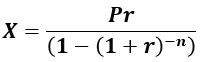
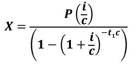
Mortgage Equation for X (constant periodic payments)
Equation 3.3 (Equation A1.5):
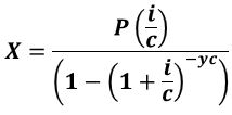
Use Equation 3.3 (Equation A1.5 in Appendix A1) to compute the constant payments based on a known loan amount, annual interest, compounding periods, and duration of loan in years.
Mortgage Equation for y (the duration of the loan in years)
Equation 3.4 (Equation A1.10):
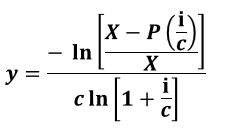
Use Equation 3.4 (Equation A1.10 in Appendix A1) to compute the loan years based on a known loan amount and known payments ,annual interest, compounding periods, and duration of loan in years.
P = principle = Present Value of all payments
X = constant payment per period
r = rate per period = i/c
i = annual interest rate (typically the “stated rate”)
c = compounding periods per year (c = 12 (monthly) , 4 (quarterly), 2 (semi-annual), and 1(yearly))
n = number of compounding periods = (c)(y)
y = number of years
Calculation Examples
I encourage you to find examples utilizing these equations on the internet. You can use an AI service (like Google Gemini) or just a traditional Google search and you’ll find many useful examples.
The examples I list below were obtained from Chapter 8.4 of an online (creative commons free share) book titled College Algebra for the Managerial Sciences by Terri Manthey (licensed under a Creative Commons Attribution-ShareAlike 4.0 International License.)
Example 3.1: Source (Terri Manthey)
You can afford $200 per month as a car payment. If you can get an auto loan at 3% interest for 60 months (5 years), how expensive of a car can you afford? In other words, what amount loan can you pay off with $200 per month? Answer (use Equation 3.2/A1.4; P = $11,120)
Example 3.2: Source (Terri Manthey)
You want to take out a $140,000 mortgage (home loan). The interest rate on the loan is 6%, and the loan is for 30 years. How much will your monthly payments be? Answer (use Equation 3.3/A1.5; X = fixed periodic payments = $839.37)
Example 3.3: Source (Terri Manthey)
Consider the $140,000 mortgage at 6% from the previous example. If the homeowner increased their payments to $1000 per month, how long will it take them to pay off the loan? Answer (use Equation 3.4/A1.10; y = the loan will be paid off in about 20 years.)
Example 3.4: Source (Terri Manthey)
If a mortgage at a 6% interest rate has payments of $1,000 a month, how much will the loan balance be 10 years from the end the loan? Answer (use Equation 3.2/A1.4; P = the loan balance with 10 years remaining on the loan will be $90,073.45)
Example 3.5: Source (Terri Manthey)
A couple purchases a home with a $180,000 mortgage at 4% for 30 years with monthly payments. What will the remaining balance on their mortgage be after 5 years? Answer ( P = The loan balance after 5 years, with 25 years remaining on the loan, will be $162,758. This one has to get solved in to steps. First compute the constant periodic payment X using Equation 3.3/A1.5, then compute P = remaining balance using Equation 3.2/A1.4 with your computed X and the remaining time on the loan = 30 – 5 = 25 years.)
The last two examples were computing remaining balances on a loan. Let’s dig a little deeper into these kinds of problems.
Remaining Balance Mortgage Equations
Schematic 4.1 below is a home mortgage payment timeline, where X are the constant periodic payments paid at the period interest rate for every period. There are a total of n periods and n payments in the loan. The initial loan is P , the principle (or Present Value PV). Bt2 represents the remaining balance at end of time t2. Time t1 is the full duration of the loan in years and time t3 is the remaining years on the loan from time t2.
Schematic 4.1 – Mortgage Payment Timeline with Remaining Balance B
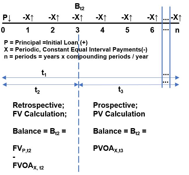
There are two methods for computing the remaining balance of a mortgage: the Retrospective Method and the Prospective Method. Refer to the timeline schematic above as you read through the sections below.
Remaining Balance Using Retrospective Method
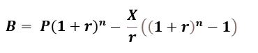
The Retrospective Method looks backwards i.e. future value calculations are required. A balance due at the end of time t2 will equal the subtraction of the future value of the Payments from the future value of the Principal:
Equation 4.1 (Equation A2.2) : Bt2 = FVP,t2 – FVOAX,t2
The first expression utilizes the Future Value Lump Sum equation and the second expression utilizes the Future Value of an Ordinary Annuity (FVOA). I cover annuities in detail (including derivations) in my blog, “Time Value of Money (TVM) Concepts, Formulas and Functions”.
If we substitute the full equations into Equation 4.1 we obtain Equation 4.2 below. Refer to Appendix 2 for more details.
Equation 4.2 (Equation A2.4):
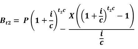
where,
Bt2 = remaining balance at end of time t2
P = present value of all payments
X = constant payment per period
r = rate per period = i/c
i = annual interest rate (typically the “stated rate”)
c = compounding periods per year
t2 = duration from time zero to Remaining Balance time.
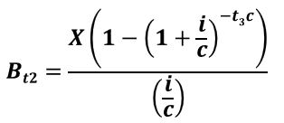
Prospective Method for Calculating Remaining Mortgage Balances
The Prospective Method looks forward i.e. present value computations are done. The remaining balance will equal the present value of the remaining payments (which is a Present Value Ordinary Annuity PVOA).
Equation 4.3 (Equation A2.5) :
Bt2 = PVOAX,t3
See my blog, “Time Value of Money (TVM) Concepts, Formulas and Functions” for more on the Present Value Ordinary Annuity PVOA equation.
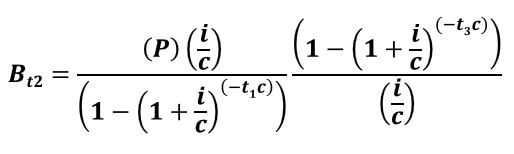
Substituting in the PVOA equation , we get Equation 4.4. Refer to Appendix 2 for more derivation details.
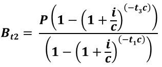
Equation 4.4 (Equation A2.6): 
If we want an expression for Bt2 in terms of the original loan (P), we can substitute for X (using Equation 3.3 and remembering that -yc = -t1c). Refer to Appendix 2 for more derivation details.
Equation 4.5 (Equation A2.9):
Where,
Bt2 = remaining balance at end of time t2
P = present value of all payments
X = constant payment per period
r = rate per period = i/c
i = annual interest rate (typically the “stated rate”)
c = compounding periods per year
t1 = full duration of loan
t3 = remaining duration of loan
Example Remaining Balance Calculations
You borrow $300,000 for 15 years at 7%. What will be the remaining balance on the loan after 6 payments?
- P = 300000; y = 15 years ; c = 12; rate = 7%/12 = .58333..
- t1c = 15 years x 12 compounding periods/year = 180, t2c = 1/2 x 12 = 6, t3c = remaining payments = 14.5 x 12 = 174
- Equation 3.3 (Equation A1.5):
- X = (300000)(7%/12) / (1-(1+7%/12)-(15)(12)) = $2,696,5
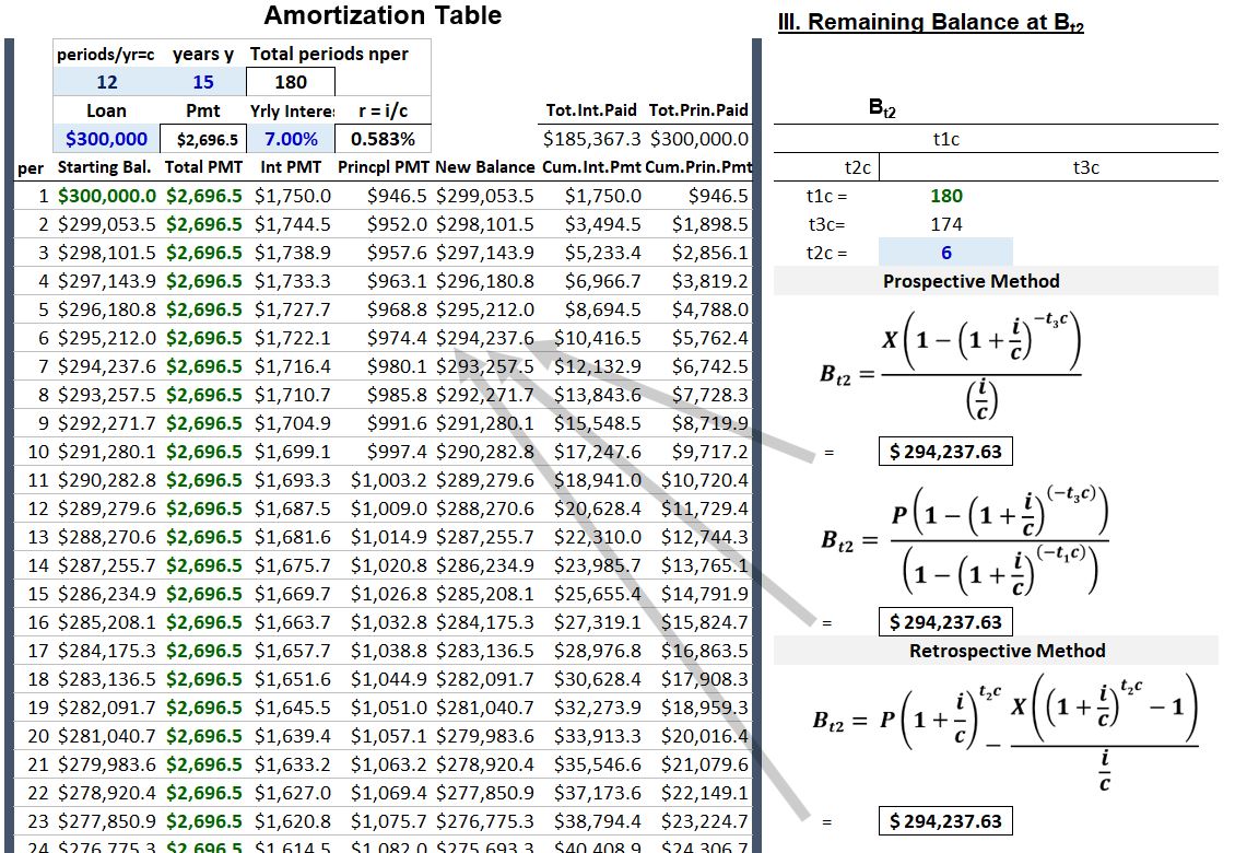
- Equation 4.2 (Equation A2.4): = (300000)(1+7%/12)(1/2)(12) – (2696.5)( (1+7%/12)(1/2)(12) – 1)/(7%/12) = 310,654.32 – 16,416.69 = $294,237.63
- Or use Equation 4.4 (Equation A2.6): = (2696.5)(1-(1+7%/12)(-174))/(7%/12) = $294,237.63
- Or use Equation 4.5 (Equation A2.9): = (300000)(1-(1+7%/12)(-174))/(1-(1+7%/12)(-180)) = $294,237.63
Financial Tools
In previous sections we established the mathematical relationships that describe most aspects of mortgage calculations. We learned that the key equations are based on
- The Present Value Ordinary Annuity (PVOA) – Mostly this one.
- The Future Value Ordinary Annuity (FVOA)
- The Future Value Lump Sum Equation
This section reviews some of the tools you can use to do mortgage calculations and shows example calculation outputs mapped to a loan amortization table.
Mortgage Equation
We’ve learned that a fixed loan mortgage is defined by the ordinary annuity equation. Typically (in the US at least), Mortgage payments are paid in arrears i.e. at the end of the period (this is what the descriptor “ordinary” implies).
With mortgages, there are 5 variables at play (note: the variables below can be written as lower case or upper case):
- number of periods = n = nper = (y)(c) where y is duration of the loan in years and c is the compounding periods per year
- interest rate per period = r = rate = i/c. These symbols are not consistently used so be careful you use the intended unit of measure (always on a per period basis).
- principal or loan amount (p or sometimes pv indicating it’s the current or present value)
- the constant and periodic payment = pmt
- the future value of the loan = fv ,which will be zero as the loan is paid off
The spreadsheet and calculator functions will require the user to establish the cash flow timing as “beginning” or “end” of period. However, in excel and on the HP 12c calculator at least, “end” of period is the default mode.
Tools
You can use a financial calculator (HP and TI make good ones) or spreadsheeting tools to compute your mortgage numbers. In the following sections we’ll review
- manual calculations in spreadsheets.
- use of Excel functions in spreadsheeting tools.
- the HP12c financial calculator functions (there are others like TI etc.).
Manual Calculations in a Spreadsheeting Tool
You can use a spreadsheeting tool like Microsoft Excel (you need to buy this) or Google Sheets (free) to build a mortgage calculator.
We already discussed how to build an amortization table but let’s do it again in a little more detail.
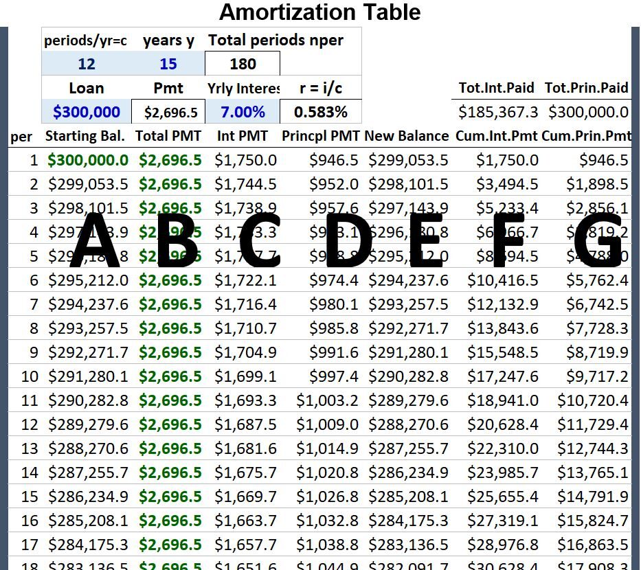
In Schematic 5.1 below, I show an amortization table for a $300,000 / 15 year loan / at a 7% annual rate/ compounded monthly.
To create an amortization table, do the following (check against the Schematic 5.1 table below as you read this):
- Given the loan (P), the yearly rate (i), the compounding period per year (c), and the loan duration in years (y)
- Compute the regular payment amount , pmt or X. Use the Present Value Ordinary Annuity Formula (PVOA) expressed for X , Equation 3.3 (Equation A1.5): = PMT = $2,696.5
- Column A = starting balance = (Starts at $300,000 and reduces by the principal portion of the payment for that period)
- Column B = fixed periodic payment = $2696.5
- Column C = interest portion of the payment for the period. For period 1 (first row) = .583% x $300,000 = $1,750
- Column D = principal portion of the payment for the period. For period 1 = B – C = $2696.5 – $1,750 = $946.5
- Column E = the new balance = remaining portion of loan = A – D = $299,053.5
- For period 2 through period 180 (15 years x 12 payments per year), repeat steps 3 through 7.
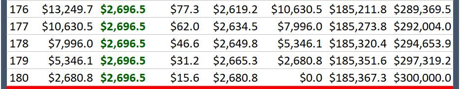
- The loan is fully paid back after payment 180 where the borrower pays back the principal ($300,000) plus an additional $185,367.3 in interest!
Schematic 5.1 – Example Amortization Table for a $300,000 15 year loan at 7% compounded monthly
note: you can download this excel spreadsheet here (2024.02.29 Mortgage Tools and Amortization Table wymhackscom.xlsx)
Continuing all the way to n = 180 payments
We could also set up and compute the remaining balance of a mortgage using our remaining balance equations (Equations 4.2 (A2.4), 4.4(A2.6), and 4.5(A2.9); see Appendix 2).
In Schematic 5.2 below I map the results of a remaining balance calculation (after 6 periods) to our example amortization table.
Schematic 5.2 – Remaining Balance Equation Outputs Mapped to Example Amortization Table.
note: you can download this excel spreadsheet here (2024.02.29 Mortgage Tools and Amortization Table wymhackscom.xlsx)
Use of Excel Functions in Spreadsheeting Tool
Microsoft Excel has several built in equations that allow you to avoid putting in and solving the applicable equations yourself. Go to Appendix 3 for more details on each of these functions.
- FV (FV(rate, nper, pmt, [pv], [type])) – Finds the future value, where
- IPMT(rate, per, nper, pv, [fv], [type]) – Returns the interest payment for a given period for an investment based on periodic, constant payments and a constant interest rate. Where,
- CUMIPMT(rate, nper, pv, start_period, end_period, type) – Returns the cumulative interest paid on a loan between start_period and end_period.
- NPER(rate , pmt, pv,[fv],[type]) – Returns the number of periods for an investment based on periodic, constant payments and a constant interest rate.
- PMT(rate, nper, pv, [fv], [type]) – PMT calculates the payment for a loan based on constant payments and a constant interest rate.
- PPMT(rate, per, nper, pv, [fv], [type]) – Returns the payment on the principal for a given period for an investment based on periodic, constant payments and a constant interest rate.
- CUMPRINC(rate, nper, pv, start_period, end_period, type) – Returns the cumulative principal paid on a loan between start_period and end_period.
- PV(rate, nper, pmt, [fv], [type]) – PV calculates the present value of a loan or an investment, based on a constant interest rate. You can use PV with either periodic, constant payments (such as a mortgage or other loan), or a future value that’s your investment goal.
- RATE(nper, pmt, pv, [fv], [type], [guess]) – Returns the interest rate per period of an annuity.
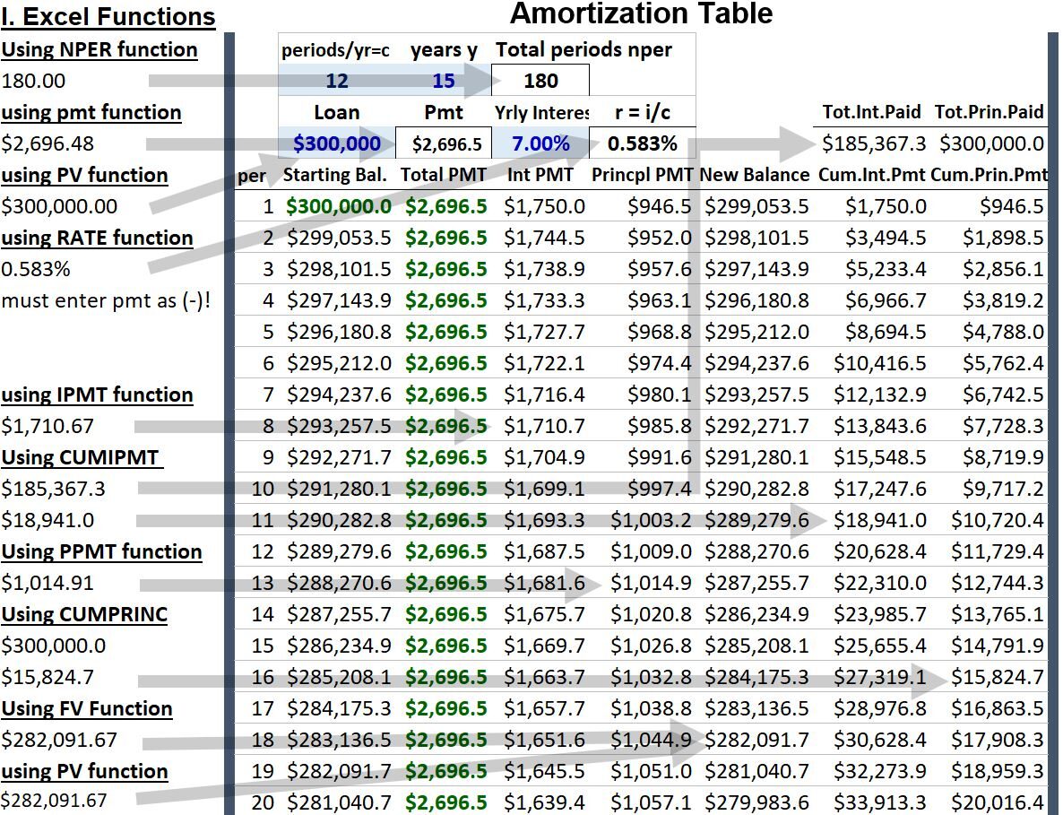
Excel Function Example Outputs Mapped to Example Amortization Table
In Schematic 5.3 below, I map example outputs of these excel functions to our example amortization table.
Remember that the pmt (constant , periodic payment) entry is conventionally entered as a negative number to indicate that it’s a cash outflow (as opposed to PV for example, which represents the loan, which is a cash inflow and has a positive sign).
Schematic 5.3 – Example Excel Function Outputs Mapped to Example Amortization Table
note: you can download this excel spreadsheet here (2024.02.29 Mortgage Tools and Amortization Table wymhackscom.xlsx)
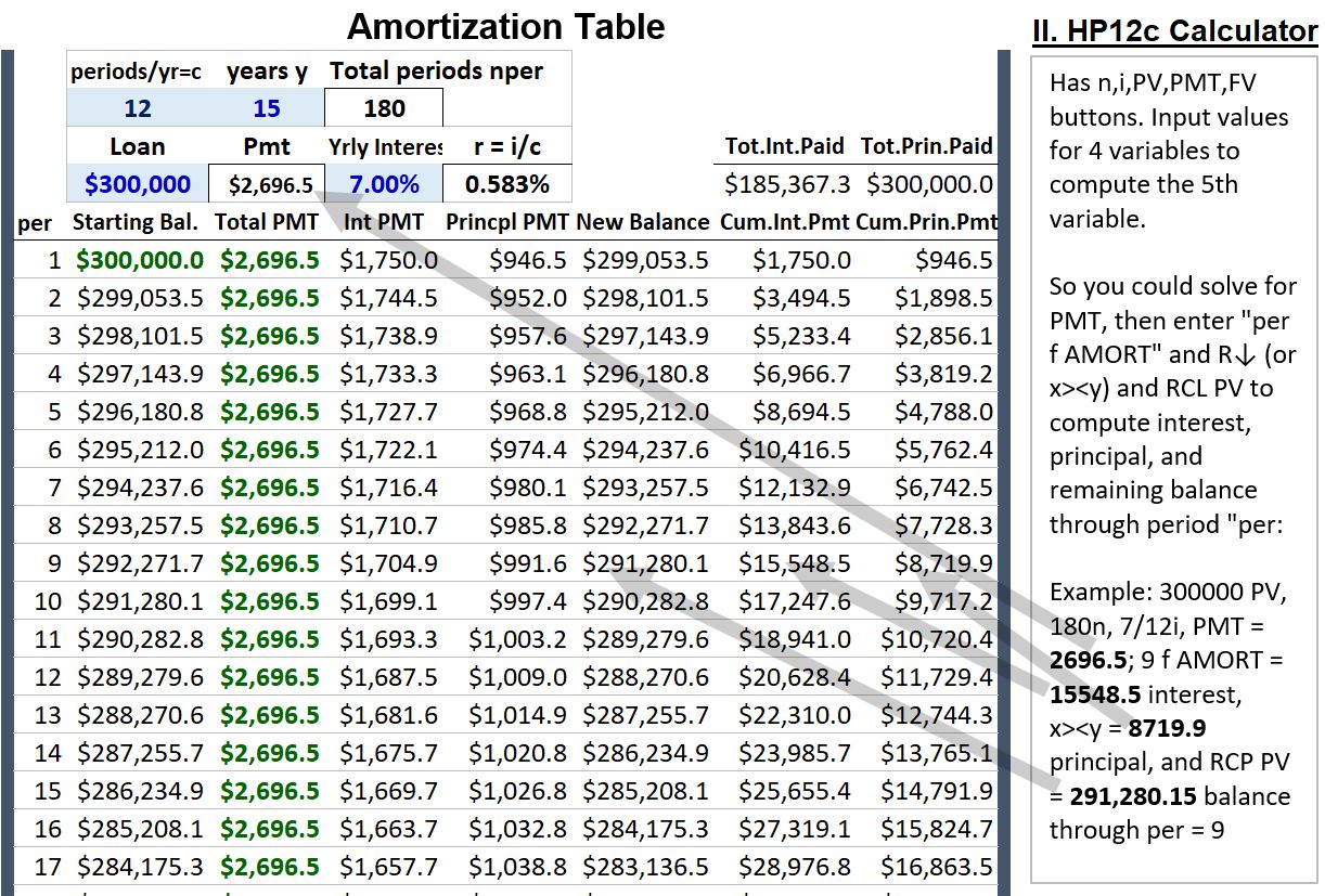
HP 12c Calculator
Check out Appendix 4 for more details on operating an HP 12c calculator. You’ll see the following 5 buttons on the calculator (note, other calculators like the TI will be set up a bit differently but the general concepts of usage are the same).
Schematic 5.4 – HP 12c Calculator Buttons

Given any four inputs, you can press the fifth button to give you your desired output. For mortgage calculations you can do the following (also see how these numbers map to the example amortization table in Schematic 5.5 below):
- Always clear registries between calculations (g REG and g FIN). Payments vs PV or FV are always going to have opposite signs. Make your pmt inputs negative to indicate cash outflow.
- Solve for PMT by entering values for n, i, pv, and fv. For example, in our amortization example from above we execute the following steps (denoting the letter means pressing the button): 18 n, .5833 i, 300000 PV, 0 FV (will default to zero but it’s a good habit to enter zero)…then press PMT to get $2696.5.
- If you press 9 f AMORT it will give you the cumulative interest through the 9th period = $15,548.5. If you press the R↓ (or x><y) button, you will get the cumulative principal payment = $8,719.9
- If instead of the above you pressed 180 f AMORT and subsequently R↓ (or x><y), you would get 185,367.3 and 300,000, the final total interest and principal paid on the loan.
Schematic 5.5 – Example HP12c Calculator Outputs Mapped to Example Amortization Table
note: you can download this excel spreadsheet here (2024.02.29 Mortgage Tools and Amortization Table wymhackscom.xlsx)
Ok, we need to wrap this up before your brain explodes.
Appendix 1 – The Mortgage Equation
The fundamental Mortgage Equation is the Present Value Ordinary Annuity (PVOA) Equation.
Consider the timeline in Schematic A1.1 below showing an “n” period mortgage where n = the duration of the loan in years y “times” the number of compounding periods per year c (i.e. n = (y)(c))
note: For typical US home mortgages, payments are normally done on a monthly basis (so there would be y x 12 payments)
Schematic A1.1 – Generic Mortgage Timeline
- A loan P (Principal) is received (cash in = + or ↓ as shown in the schematic above).
- Constant and periodic cash payments X are made (cash out = – or ↑).
- At the end of the loan (the nth payment), the FV of the loan becomes 0 (its been paid off)
The mathematical expression for fixed rate mortgages is the Present Value Ordinary Annuity (PVOA) equation (we can call this the Mortgage Equation as well).
Equation A1.1 :
P = present value of all payments
X = constant payment per period
r = rate per period = i/c
i = annual interest rate (typically the “stated rate”)
c = compounding periods per year
n = number of compounding periods = (c)(y)
y = number of years
Equation A1.2:
Equation A1.3:
Clean up the Right Hand Side a little bit to get:
Equation A1.4:
Substitute the expressions for r and n into Equation A1.2 to get:
Equation A1.5:
Equations A1.4 and A1.5 are the explicit forms of the Mortgage equation for P and X.
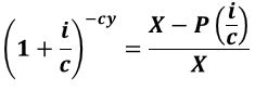
We also want an expression for y (the duration in years of the loan) as well. Equation A1.4 can be expressed as:
Equation A1.6:
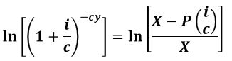
Equation A1.7:
Equation A1.8:
Equation A1.9:
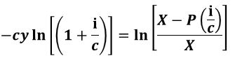
Equation A1.10:
Summary
Mortgage Equation for P (Principal or Loan Amount)
Equation A1.4:
Mortgage Equation for X (constant periodic payments)
Equation A1.5:
Mortgage Equation for y (the duration of the loan in years)
Equation A1.10:
P = present value of all payments
X = constant payment per period
r = rate per period = i/c
i = annual interest rate (typically the “stated rate”)
c = number of compounding periods per year
n = number of compounding periods = (c)(y)
y = number of years
Appendix 2 – Mortgage Remaining Balance
In the previous section, we established mortgage equations expressing the Principal (or loan) P , the Payment X, and the duration of the loan y.
Another useful computation is finding out the Remaining Balance of a loan i.e. at some point before the loan is fully paid off.
In the Schematic A2.1 below, consider annual fixed payments X, that pay back a loan P in n periods (n periods = duration of loan in years y “times” the number of compounding periods c = (y)(c)). We want to compute the balance owed (Remaining Balance) after t2 years Bt2.
The durations t1 , t2, and t3 describe the full loan duration, the duration at which the Remaining Balance is computed , and the duration remaining from the time in which the Remaining Balance is computed.
That’s a mouthful! Just look at Schematic A2.1 below.
Schematic A2.1
There are two methods used to calculate the Remaining Balance on a mortgage. These are described in the following sections. Refer to Schematic A2.1 as needed.
Retrospective Method for Calculating Remaining Mortgage Balances
The Retrospective Method looks backwards i.e. future value calculations are required. A balance due at time t2 will equal the subtraction of the future value of the payments from the future value of the Principal:
Equation A2.2: Bt2 = FVP,t2 – FVOAX,t2
We can make Equation A2.2 more explicit by using the Future Value Lump Sum equation and the Future Value Ordinary Annuity (FVOA) equation. If you want to learn more about these and how they are derived, refer to my blog “Time Value of Money TVM Concepts Formulas and Functions“.
Equation A2.3:
B = remaining balance
P = present value of all payments
X = constant payment per period
r = rate per period = i/c
i = annual interest rate (typically the “stated rate”)
c = compounding periods per year
n = number of compounding periods = (c)(y)
y = number of years
Substituting for r = i/c and n = yc , n = t2c we get:
Equation A2.4:
where
t2 = duration from time zero to Remaining Balance time.
Prospective Method for Calculating Remaining Mortgage Balances
The Prospective Method looks forward i.e. present value computations are done. The Remaining Balance will equal the Present Value of the remaining payments.
Equation A2.5: Bt2 = PVOAX,t3
Let’s make Equation A2.5 more explicit.
Equation A2.6:
Equation A2.7:
Substitute Equation A2.7 into Equation A2.6 to get:
Equation A2.8:
or
Equation A2.9:
Where,
Bt2 = remaining balance at end of time t2
P = present value of all payments
X = constant payment per period
r = rate per period = i/c
i = annual interest rate (typically the “stated rate”)
c = compounding periods per year
t1 = full duration of loan
t3 = remaining duration of loan
Appendix 4 – Calculator Functions
I am excerpting this section from my blog, “Time Value of Money (TVM) Concepts, Formulas and Functions”.
Also refer to the Boston Inst of Finance common keystrokes for more instructions and examples using the HP 12c calculator.
TVM Calculations Using a Financial Calculator
Your financial calculator can do single cash flow and Annuity (equal value and equal period cash flow) discounting and compounding calculations. It can also do NPV calculations.
Single Cash Flow and Annuity Calculations
Where
Solving for a Particular Variable
Loan Calculations
Loans (debt repayments) are typically Ordinary Annuity type calculations. Your financial calculator has a few additional keys to help you do these kinds of calculations.
Example: You take out a $200,000 home loan (30 year fixed; interest rate of 3%; monthly mortgage payments). What is the monthly mortgage payment and how much interest will have been paid after 5 payments?
- Key entries on the HP 12c: n = 30×12=360, PV=$200,000,i = 3/12=.25,FV=0.
- Pressing the PMT key gives – $843.21 = the monthly mortgage payment.
- Pressing “360 f Amort” gives -103,554.9 the total interest paid and
- Pressing the R↓ key gives -200,000, the principal paid (note: The R↓ and x><y buttons are interchangeable i.e. you get same result)
- Pressing the buttons RCL and PV will give the remaining balance (which is 0 of course)