Last Revision: September 29,2022
Introduction
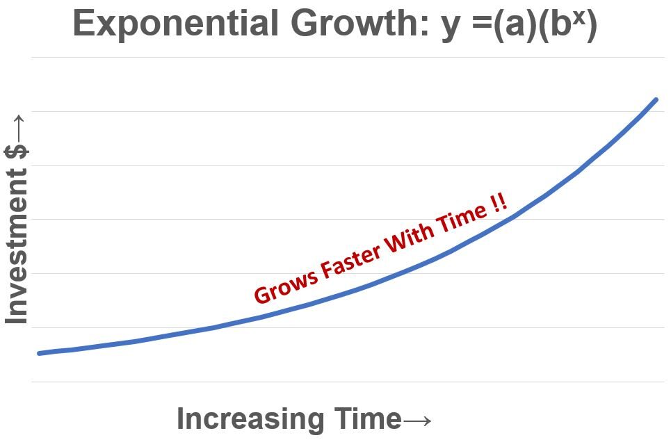
The power of compounding allows money to grow exponentially over time. That is, over time, the growth accelerates! So start investing (for yourself or your kids) as early as possible to maximize the amount of money you’ll have in the future.
Schematic 1: Compounding – (a) grows exponentially by (bx)
In this post we’ll go through some examples showing how investments grow exponentially over time and why it’s so important to start investing as early as possible. We’ll also show how expenses (fees), taxes, and inflation work against this growth. Refer to Appendix 1 and Appendix 2 to see how the Compounding Formula and Ordinary Annuity formulas are calculated. The Annuity formula, which is used in the compounding calculator, is a version of the compounding formula when periodic investments are made. Use the buttons below to navigate this post.
Power of Compounding Example 1 – Time
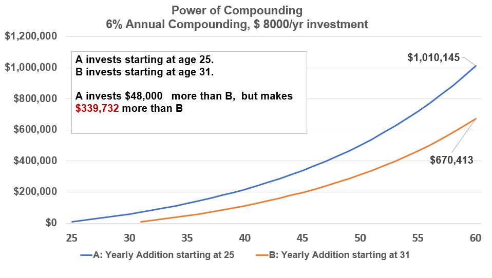
Person A starts investing at 25 years of age and invests $8,000 every year to age 60. Person B, starts at 31 years of age and also invests $8,000 every year to age 60. They both get a 6% compounded annual return.
By starting at an earlier age, Person A makes about $340,000 more than Person B.
Graph Example 1 – Power of Compounding – Start Time
Power of Compounding Example 2 – Time (Start/Stop)
Compounding Example 2a.
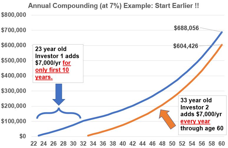
The example in Graph Example 2a below shows how powerful time is with respect to compounding. It compares the future value of investments made by two investors. The first investor has just graduated college and started her first job. She invests $7,000/year for only the next 10 years and then stops investing any more money. The blue line charts the growth of her investment through age 60. A second investor also starts working at 23 but he doesn’t invest any money until age 33, but from 33 until he retires at age 60, he invests $7,000 every year. The orange line charts the growth of his investment through age 60. Compare the final investment values at age 60!
Graph Example 2a: Power of Compounding – Timing
Graph Example 2a Observations and Lessons:
- Investor 1, having invested $7,000 x 10 = $70,000 over only the first 10 years has grown her investment at age 60 to ~$688,000
- Investor 2, having invested $7,000 x 28 = $196,000 over 28 years (but started 10 years later than investor 1) has grown his investment to about ~$604,400
- Investor 2 made $83,600 LESS than Investor 1 but invested $126,000 MORE!
- The accelerating effects of compounding over time make it crucial that you invest as early as you can! Time is the critical factor.
- Since this example is assuming annual periodic investments, the proper equation to use is the Annuity formula. Refer to my post on the Power of Compounding for a derivation of the annuity equation.
Compounding Example 2b.
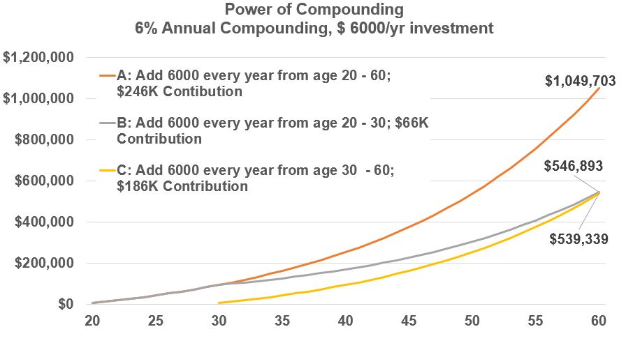
Investors A, B, C invest $6,000 per year and receive a 6% return compounded annually. Person A and B start investing at 20 years of age. Person A adds money each year all the way to the final year (age 60). But Person B stops adding after age 30. Person C starts at 30 and adds money each year till age 60.
Start early is the message!! Person C had to make a lot more contributions ($186K versus Person B’s $66K) to get to about the same future value that B got.
Graph Example 2b – Power of Compounding – Start and Stop Time
Power of Compounding Example 3 – Fees
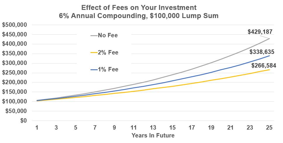
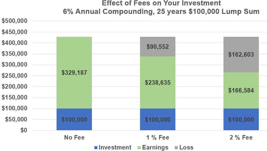
You make a lump sum investment of $100,000 and it grows at 6% compounded annually. In one instance, you pay no fees which is not a practical assumption because you will pay fees. In the other two scenarios, you pay a 1% annual fee or a 2% annual fee. Assume that the fee is structured as an expense ratio (based on your total assets).
A 1% annual fee reduces your earnings by about 21%.
A 2% annual fee cuts your earnings by 38%.
See the line graph and the bar graph below showing these differences.
Don’t let the small percentage numbers fool you! The long term value destruction is huge. If you are investing in mutual funds or ETFs, I think its reasonable to keep your expense ratios below one. Consider investing in Index Funds (ETFs or Mutual Funds) where expense ratios can be below .1% (yes; point 1%).
So, based on your specific situation, minimize your investment fees!
Graph Example 3(a) – Power of Compounding – Fees – Line Chart
Graph Example 3(b) – Power of Compounding – Fees – Bar Chart
Power of Compounding Example 4 – Inflation
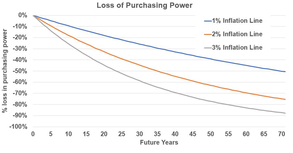
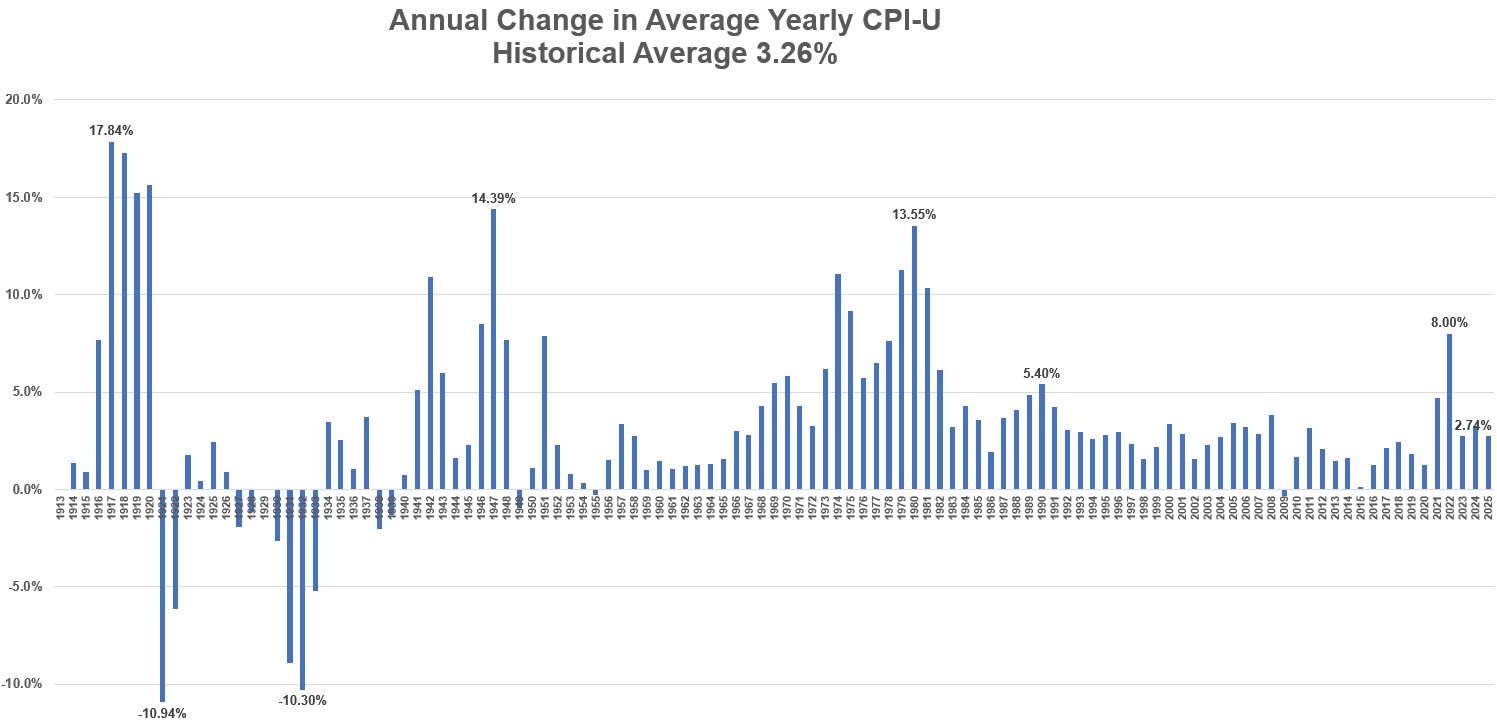
A dollar today (typically) is worth less in the future i.e. we typically have inflation in our economy. (see Graph 4(c) below)
You can use the Compounding Equation to determine the loss of purchasing power of the dollar due to inflation
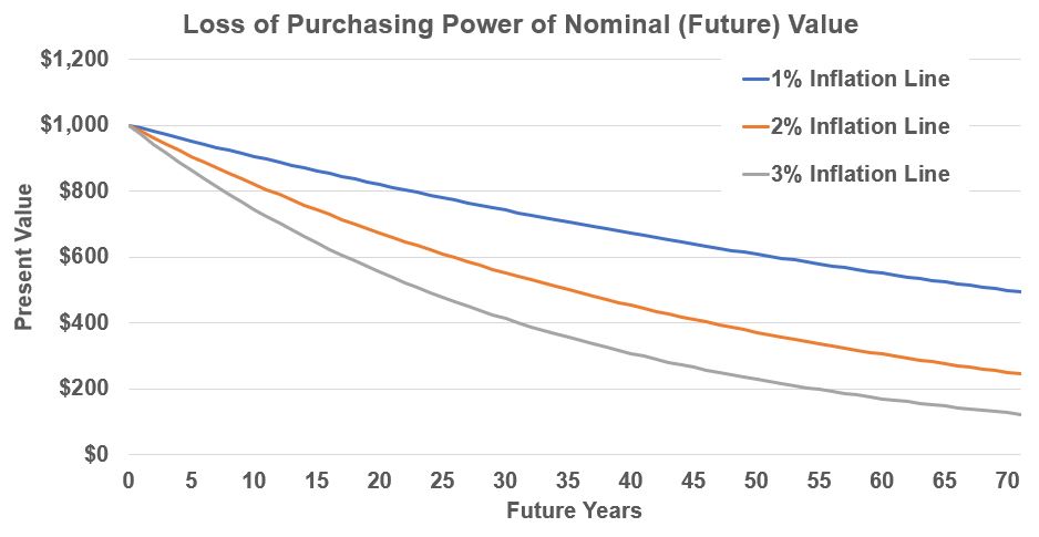
Again don’t let the small percentages fool you (See Graph 4(a) and Graph 4(b) below). For example after 25 years, a 3% inflation rate will reduce the value of the dollar by over 50% !
To understand the purchasing power of the dollar, use the compounding equation to convert the future value into a present value. Sometimes the present value is referred to as constant dollars.
PV = FV/(1+inflation rate)^n
Graph_Example_4(a) – Loss of Purchasing Power in Percentages
Graph_Example_4(b) – Loss of Purchasing Power of $1000 over time
Graph_Example_4(c) – Historical Inflation Rate (source: BLS)
Power of Compounding Example 5 – Total Costs
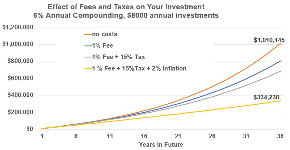
In reality, your investment value will be reduced by the combination of fees, inflation, and taxes. Lets consider one more (realistic) example in the chart below where all expenses are incurred.
A 25 year old person invests $8,000 every year for 36 years at a 6% compounding annual return. Lets assume that the yearly costs will be 1% fees, 15% taxes, and 2% inflation each year.
The ideal no-cost value of $1,010,145 will be reduced to a value of $334,238 (that is a 67% reduction!)
Maximize your compounding investments by Starting Early and Minimizing Your Expenses!
Graph Example 5 – Power of Compounding – Impact of Fees, Taxes, Inflation
Power of Compounding Example 6 – Growth at Different Rates
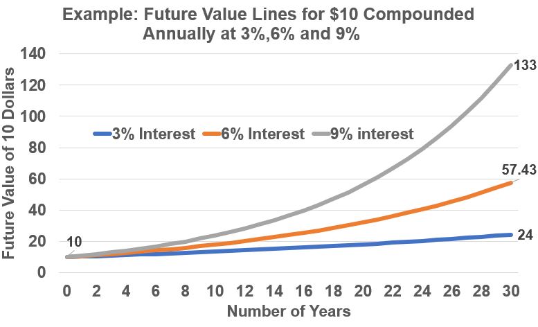
Graph Example 6 shows the future value of 10 dollars growing at different annual compounding rates. Please notice two very important characteristics:
- The growth ACCELERATES with time (i.e. the slope of the curve changes and gets steeper)
- The higher the interest rate the steeper the curve over a certain time period
Graph Example 6: Growth of 10 Dollars Compounded Annually
Appendix 2 – Ordinary Annuity Equation Derivation
See this video for a nice step by step derivation of the Ordinary Annuity Equation.
Let’s derive the Periodic Investment Compounding Formula (the Ordinary Annuity Equation) below.
Consider an n year investment where a constant P dollar quantity is being added at the end of each period.
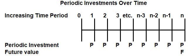
We want to know the future value F of our investment if we assume we get a i % yearly compounded return.
Let’s compute F by adding up each period’s contribution. Add them up from right to left:
P +
P(1+i)^1 +
P(1+i)^2 +
P(1+i)^3 +
etc.
P(1+i)^(n-3) +
P(1+i)^(n-2) +
P(1+i)^(n-1)
The above is a geometric series because you can divide consecutive terms and get the same value:
i.e. P(1+i)^1 / P = 1+i , and P(1+i)^2 / P(1+i)^1 = 1+i
Formula for a Geometric series
S = a (r^n – 1)/(r-1)
Substitute P for a and (1+i) for r in equation above
F = P ( (1+ i)^n -1 ) / (1+i -1)
F = P ( (1+ i)^n -1 ) / i (Ordinary Annuity)
Where, P = periodic payment
i= effective interest rate
n= number of periods
Note1 : If we express i as the Annual Percentage Rate, then
(1+i)^n becomes (1+i/c)^cn
Note2: If the first investment is made at the beginning of the periods, then
F = (1+i) P ( (1+ i)^n -1 ) / i (Annuity Due)