Simple Interest
Consider the following scenario:
You invest an amount P in a bank savings account. The bank will pay you 2% Simple Interest annually. How much money will you have after 3 years?
After 3 years, you will have P +2%P + 2%P + 2%P = P(1+(3)(2%)).
We can expressed this generally as: F = P(1+nr) = Simple Interest Formula
Table 1: Simple Interest Formula
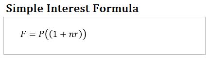
- F = P(1+nr)
- F = Future Value,
- P = Present Value,
- n = total number of periods
- r = Interest rate per period
- note that the same period unit has to be used for n and r
- This is called the Simple Interest Formula
Some examples where simple interest is used:
- Corporate bond interest payments (coupon payments)
- Auto loans
- Certificates of deposit
- Federal student loans
- Most private student loans
- Short term loans
Compound Interest
Now, let’s use the same example we used for simple interest but with a twist.
This time, you invest an amount P, and the bank offers you 2% interest Compounded Annually for 3 years.
This means you’ll get “interest on your interest”.
After 1 year, your investment will be worth:
P + 2%P = P(1+2%).
After the 2nd year your investment will be worth:
P(1+2%) + P(1+2%) x 2% = P(1+2%)(1+2%)
And after the 3rd year your investment will be worth:
P(1+2%)(1+2%) + P(1+2%)(1+2%) x 2% = P(1+2%)(1+2%)(1+2%)
We can express this generally as:
F = P(1+r)n = Compound Interest Formula for a Single Cash Flow.
The formula can be expressed in four ways depending on the variable that needs to be computed (see the equations in the box below).
Table 2 – Single Payment Compound Interest Formulas and Factors
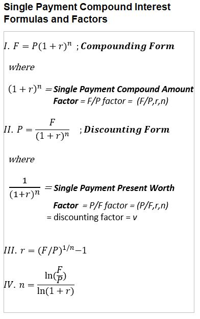
Where:
- F = P(1+r)n = P(1+i/c)cy
- F = Future Value, P = Present Value,
- i = yearly interest rate (sometimes called the stated rate)
- c = number of compounding periods per year
- r = interest rate per compounding period = i/c
- y = number of years
- n = total number of compounding periods = (c)(y)
- This is called the Compound Interest Formula for a Single Cash Flow
If you want to derive Equations III. and IV. above from I. , remember your logarithm and exponent rules:
- ln ab = ln a + ln b
- ln a/b = ln a – ln b
- ln ab = b ln a
- (ab)1/b = a
- ln(1) = 0
Compounding is Everywhere
Some places where compounding is at work are:
- Bank savings and money market accounts
- Stock investments
- Compound interest on credit card overdue amounts (paying interest on overdue credit card amounts is bad news since interest rates here tend to be very high).
- Certain government bonds (EE, I, Zero Coupon).
How the Lump Sum Compounding Formula Can Be Used
In the equation, F = P(1+r)n = P(1+i/c)cy , You can solve for any variable F, P, r = i/c , n= (c)(y) as long as you know the other three.
- Example: Solve for what your investment will be worth in the future.
- Example: Solve for what you need to investment now to earn a future amount.
- Example: Solve for how long it will take your investment to grow a target amount
- Example: Solve for your investment rate of return.
The Power of Compounding
The exponential component of compound growth allows your investment returns to accelerate over time.
Every investor should know that it’s important to invest early and let time work for her/him.
Check out my post on the power of compounding.
The Good and the Bad
Compounding is also a “double edged sword”.
Compounding works for you in investing but can work against you when you borrow!
An alarming example is the current US Federal Government Interest payments on the debt.
Another example that might hit closer to home is credit card debt (interest rates can get really high…they are 20% and “change” as I write this on Feb 13, 2024).
The Compounding Formula is Foundational
The compounding formula, F = P(1+r)n = P(1+i/c)cy is the Foundation of most Time Value of Money (TVM) Calculations.
This will be more evident in later sections when we discuss multiple cash flow scenarios (Annuities, Perpetuities, and irregular cash flows).
Continuous Compounding, Effective Annual Rate, and Equivalent Rate
In the compounding formula, F = P(1+i/c)cy = P(1+r)n , while the stated interest rate (i) is a certain value, the actual or effective interest might not be the same.
It depends on the frequency of compounding (c).
Consider the Compounding Equation for a Single Cash Flow, F = P(1+i/c)cy = P(1+r)n
Let
- F = Future Value
- P = Present Value
- y = number of years
- i = annual interest rate (typically the “stated rate”)
- c = compounding periods per year
- r = rate per period = i/c
- n = number of periods = (c)(y)
- Compounding Factor = (1+i/c)cy = (1+r)n
- e = Euler’s number = 2.71828…
- EAR = Effective Annual Rate
If the compounding is done more frequently than annually (i.e. semi-annually, quarterly, etc.), the actual annual interest rate (or Effective Annual Rate or EAR) will be higher.
Consider the Table 3 example below.
Table 3 – Continuous Compounding and Effective Annual Rate Example
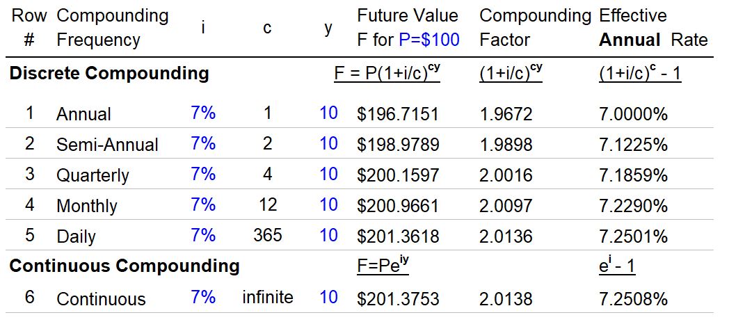
Table 3, shows the future value of $100 (P) invested for 10 years (y) at a 7% stated annual interest rate (i) for different compoundings (c) per year.
As the compoundings increase from row 1 to 6 in the table, so does the future value (from $196.7 to $201.38).
We see that:
- As the number of compoundings per year go towards infinity, the future value equation for discrete compounding F=P(1+i/c)cy becomes the equation for Continuous Compounding F = Peiy (where e = Euler’s number = 2.71828…; which is a non-terminating irrational number).
- Euler’s number is fascinating. See Appendix 24 for more on Euler’s number and the derivation of the continuous compounding formula.
- As the yearly compounding periods increase, the actual annual interest rate (or Effective Annual Rate) gets increasingly larger than 7% (the stated annual compounding interest rate).
- The Effective Annual Rate (EAR) is simply the annual compounding factor minus 1 (the 1 converts it to a fraction or percent) or (1+i/c)c-1.
- For example, for annual compounding, the EAR is 7% while for monthly compounding the EAR is actually 7.23%. At the limit (when c is infinite), the EAR is 7.25%.
Equivalent Rates
It’s useful to know how to express an annual rate as the equivalent rate per period
So, if I have an annual rate of “a” , how can I express this as an equivalent quarterly or semi-annual or monthly rate?
We can develop a useful formula with an example.
Example: If the annual rate is a%, what will be the equivalent rate if we compounded quarterly? Assume an investment of 100.
- We want to know the equivalent quarterly rate that will produce the same future value as the annual rate.
- 100(1+a)=100(1+quarterly rate)(1+quarterly rate)(1+quarterly rate)(1+quarterly rate)
- 100(1+a) = 100(1+quarterly rate)4
- Solve for quarterly rate: quarterly rate = (1+a)1/4-1
We can generalize this formula to: (1+a)1/c-1 = period c rate.
So for example, if the annual rate is 6% and the compounding is actually quarterly, then the equivalent rate is (1.08)^(1/4)-1 = 1.94%.
Summary
Continuous Compounding Formula: F = Peiy
The Compounding Formula becomes the Continuous Compounding Formula when there are an infinite number of compounding periods, c.
Effective Annual Rate: EAR = (1+i/c)c-1
A periodic rate, c ,can be expressed as an Effective Annual Rate using this formula.
Equivalent Rate: (1+annual rate)(1/c) – 1 = period rate
An annual rate can be expressed as an equivalent periodic rate with this formula.
where,
- F = Future Value
- P = Present Value
- y = number of years
- i = annual interest rate (typically the “stated rate”)
- c = compounding periods per year
- r = rate per period = i/c
- n = number of periods = (c)(y)
- Compounding Factor = (1+i/c)cy = (1+r)n
- e = Euler’s number = 2.71828…
- EAR = Effective Annual Rate
Using a Timeline
We want to develop the compounding formula for multiple cash flows, but ,before we do, let’s discuss a very useful construct that can help you visualize the value of money across time: the timeline.
It’s a best practice to draw out a timeline when you do Time Value of Money calculations.
In simple examples, this will seem trivial but in more complex scenarios it will help you set up the problem correctly and avoid making mistakes.
Consider Schematic 1 below:
Schematic 1 – TVM Timeline
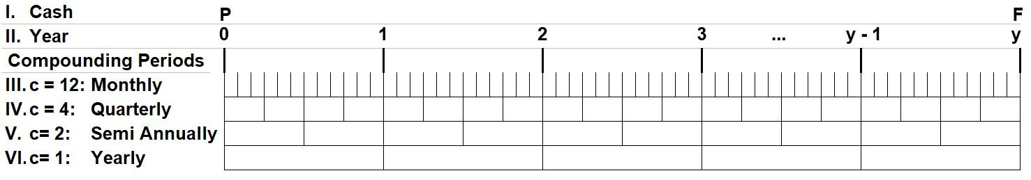
- The timeline has labeled rows I. through VI. The Cash Row (I.), shows the Present Value, P (todays value), the Future Value, F.
- note: We will address periodic payments/investments in the next section where additional cash occurs in between (and including) P and F.
- The Year row (II.) shows the year counters starting from today(0) and going to y years
- The compounding periods, c , are shown for c = 12 (monthly) , 4 (quarterly), 2 (semi-annual), and 1(yearly) periods
Lets do a couple of examples using the Compounding Formula for a Single Cash Flow: F=P(1+r)n
Single Cash Flow (Lump Sum) Future Value Calculation
Example 1: Invest $10,000 today, at 4% compounded semiannually for 5 years. What is the future value?
Remember that r = i/c and n = (c)(y) and annual, semi-annual, quarterly, monthly, and daily periods would be 1,2,4,12,365 respectively.
- P = $10,000
- i= 4%
- c = 2 ; semi annual means compounding is twice per year
- r = i/c = 2%; we must adjust the annual rate i by the number of compounding periods
- y=5 years
- n =(2)(5)=10 compounding periods
- F = 100(1+2%)10 = $12,189.9
Single Cash Flow (Lump Sum) Present Value Calculation
Example 2: The Value of your investment in 5 years, if compounded monthly at 3%, is $13,000.
What is the current or present value of this investment?
- F = $13,000
- i=3
- c = 4
- r=i/c=.75%
- y = 5
- n=(4)(5)= 20
- F=P(1+r)n , therefore, P = F/(1+r)n
- P = 13,000/(1+.75%)20= $11,195.5
In other problems you might need to solve for r or n as well and this is easily done as long as you know the other three variables.
Compounding and Discounting
The timeline concept helps us intuitively understand two commonly used TVM terms.
- When we compute the future value , we are Compounding the present value P into a future value F.
- This term is intuitive as it suggest growth of the present value into a larger future value.
- When we compute the present value from a future value we describe this as Discounting the future value.
- This term is intuitive as well and implies a reduction. The present value will be a smaller value than the future value.
All the examples so far assume there is a one time investment at time zero.
What happens when we have additional investments (or withdrawals) that occur in between the beginning and the end? Read on.
Multiple Cash Flows
In the previous section we reviewed two examples where we computed the Present and Future value of a single investment (no additional investments were assumed).
Now consider a few more examples where we make more than one investment. This is where drawing a timeline is very useful.
Multiple Cash Flows, Future Value Calculation
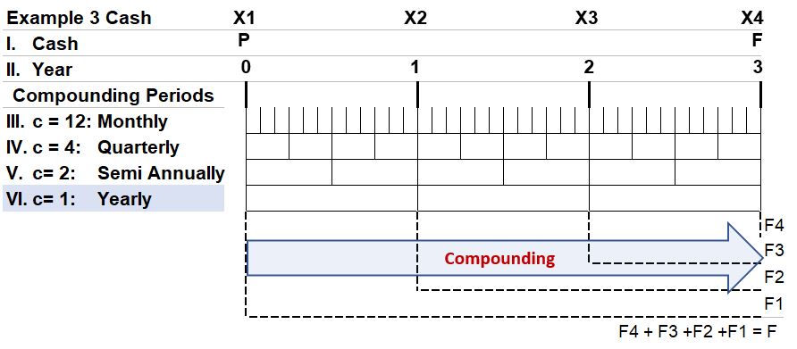
- These investments occur in different years. In order to express them all as a single future value, we have to adjust the values of each cash flow by the time remaining and the interest rate.
- The future value will therefore be the sum of the individual investment future values. We’ve applied the Cash Flow Additivity Principle here i.e. we can adjust each flow individually and then add them up.
- F = X4 + X3(1+6%)1 + X2(1+6%)2 + X1(1+6%)3
- Note!!! Due to the additivity principle, each term stands by itself.
- That means that the cash flows could be the same , different, periodic , or not (irregular or un-even). It doesn’t matter.
- You simply take each cash flow and adjust them accordingly to express all of them as a singular future value cash flow.
Schematic EG3.1 – TVM Timeline with Multiple Cash Flow Compounding Example
Multiple Cash Flows, Present Value Calculation
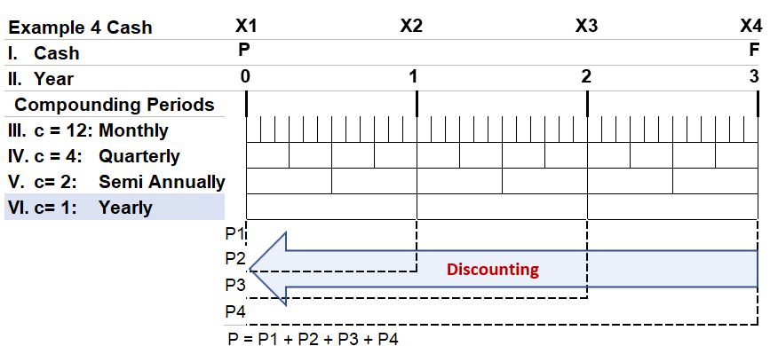
- The present value will be the sum of the individual investment present values.
- This time we’ll use the discounting form of the Compounding Formula.
- P = X1 + X2/(1+6%)1 + X3/(1+6%)2 + X4/(1+6%)3
- Note!!! Due to the additivity principle, each term stands by itself.
- That means that the cash flows could be the same , different, periodic , or not (irregular or un-even). It doesn’t matter.
- You simply take each cash flow and adjust them accordingly to express all of them as a singular present value cash flow.
Schematic EG4.1 – TVM Timeline with Multiple Cash Flow Discounting Example
Direction of Cash Flows
Any cash flow should be defined as an inflow (being received) or an outflow (an expense, payment, or an investment).
If you do financial calculations in a spreadsheet like excel or on a financial calculator, you will have to input cash outflows as negative (-) values and cash inflows as positive values.
For single (lump sum) cash flows, PV and FV will have opposite signs.
For example, if you invest $10,000 today, what will the future value be if it compounds annually at 7% for 10 years. The answer will be $-19,671.51 if you input the PV as +$10,000 (if you had input the PV as negative, the FV output would be positive.).
This becomes more important when you do multiple cash flow calculations.
Now you have three variables that assume either a positive or negative value (the present value, the future value, and the periodic cash flow). The periodic cash flow must have the proper sign.
Cash Inflow (+) Examples:
- income (pension, paycheck, savings income etc.)
- borrowed money like a home mortgage or auto loan
Cash Outflow (-) Examples:
- payments (debt, educational, purchases)
- investments (outflow from you that hopefully results in return inflows)
TVM Calculations Rules (Principles)
Let’s recap…Examples 3 and 4 showed multiple cash flows.
We computed a singular future or present value of the cash flows by applying the compounding (or discounting) equation to each cash flow (using the appropriate time period and given interest rate).
The Additivity Principle allows us to (a) convert each cash flow to the appropriate time at a given interest rate and then (b) sum them all up to get the singular present or future value.
In scenarios with multiple cash flows like Examples 3 and 4 above, you must ALWAYS convert the cash flows across multiple periods back to a singular period.
You have to do this to normalize the effects of time. Make sense, right? You cannot compare 2016 dollars with 2022 dollars for example.
You need to adjust one or the other so they are expressed on the same basis.
So, two fundamental tenets of TVM calculations are:
- You have to express multiple cash values on the same basis (PV or FV) if you are going to do any comparison or evaluation
- You need to account for the direction of Cash flow. Cash outflow (think expenditures or investments) inputs into calculator or spreadsheet tools are assumed to be negative.
Example 5: Write out the Present Value equation for a cash flow scenario where in year zero an investment of C (call it Co) occurs and at the end of the next 3 years income P1, P2 and P3 (respectively) are earned. The annual interest i is compounded quarterly and the income is paid annually and at mid year.
- PV = C0 + P1(1+i/c)(cy1) + P2(1+i/c)(cy2) + P3(1+i/c)(cy3)
- Income paid annually and at mid mid year means P1 occurs at year .5 , P2 occurs at year 1.5, etc.
- Note that if cash flow timing was end of year, then y1 = 1, y2 = 2, etc.
- c = 4; cy1 = (4)(.5)=2, cy2 = (4)(1.5)=6, cy3 = (4)(2.5)=10
- PV = -C0 + P1(1+i/4)2 + P2(1+i/4)6 + P3(1+i/4)10
- Note that Co is entered as a negative value because its a cash outflow
- Note that the P expressions are expressed positively because they are cash inflows.
We will revisit the example 4 and 5 equations in later sections when we discuss DCF (discounted cash flow), NPV (net present value) and un-even cash flows, but we want to talk about Annuities first.
Annuities and Perpetuities Defined
So far we have only considered the compounding or discounting of single investments at time P or F respectively.
Annuities and Perpetuities involve multiple cash flows that compound over time.
Formulas for Annuities and Perpetuities are based on the compounding and discounting forms of the Compound Interest Formula P = (1+r)n. (see how in the derivations located in the Appendices 3- 14.).
Annuities are constant (or constantly growing) and even (equal interval), periodic cash flows that occur (typically) weekly, monthly, quarterly, or yearly .
They last for a finite period of time. These are employed in all sorts of financial calculations (e.g. investments, retirement planning, mortgages and other loans, education cost planning, etc..).
Perpetuities are Annuities with infinite cash flows.
These don’t sound very useful but are often used by corporations and financial firms to estimate end of project ( liquidation or terminal or going concern) values.
The perpetuity concept can be also applied to rents on property investments or dividends on stocks to value those assets.
Annuities/Perpetuity Types Defined on a Timeline
Consider Schematic 2 below where we have periodic cash investments over a three year period.
Some are constant over time while others grow geometrically at a yearly growth rate g (or grow arithmetically at a constant G) .
Schematic 2 – Annuities Defined on a 3 Year Timeline (note: For infinite periods, the exact definitions apply to Perpetuities as well)
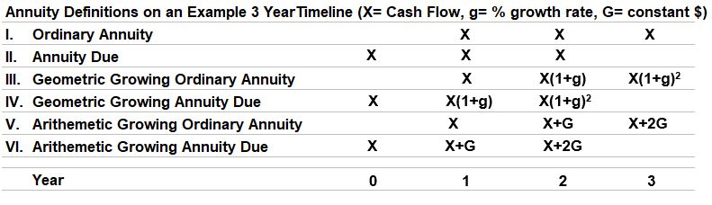
An Ordinary Annuity (or Perpetuity for infinite periods) has its first cash flow occur at the end of the period.
- e.g. In Schematic 2 row I., periodic cash amount X starts at end of year 1 and is added with the same timing in subsequent years.
An Annuity (or Perpetuity for infinite periods) Due has its first cash flow occur at the beginning of the period.
- e.g. In Schematic 2 row II., periodic cash amount X starts at the beginning of year 1 (at year =0) and is added with the same timing in subsequent years.
Growing Annuities/Perpetuities
A Geometrically Growing Ordinary Annuity (or Perpetuity for infinite periods) has cash flows that evenly grow over time at a fixed growth rate starting at the end of the period.
- e.g. In Schematic 2 row III., X starts at the end of year 1, grows to X(1+g) at the end of year 2 etc. (g is a fixed growth rate percentage)
A Geometrically Growing Annuity (or Perpetuity for infinite periods) Due has cash flows that evenly grow at a fixed growth rate beginning at the start of each period.
- e.g. In Schematic 2, row IV., X starts in year 0, then grows to X(1+g) at the beginning of year 1, etc.
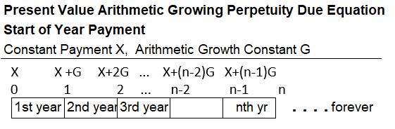
Arithmetically Growing Annuities/Perpetuities have similar definitions (for Ordinary Annuity and Annuity Due) but the growth in this case is linear by a constant G (X, X+G, X+2G etc.)
Refer to the Appendices for detailed annuity equation derivations.
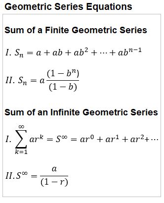
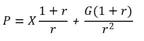
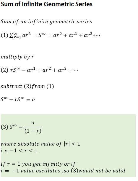
Sum of a Geometric Series
The formulas for the sum of a finite or infinite Geometric series (formulas II. in the box below) are used in the derivation of annuity formulas. Refer to Appendix 2 and Appendix 3 for their derivation.
Table_4 – Finite Geometric Series Formula
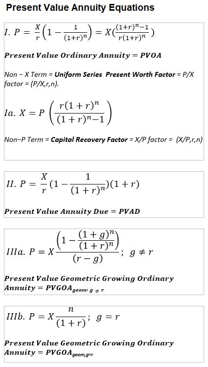
Present Value Annuity Formulas
Table 5 – Present Value Annuity Formulas
Variable Definitions
- P = Present Value
- X = Periodic Payment
- i = annual rate (expressed as fraction)
- c = compounding periods per year
- r = rate per period = i/c (expressed as fraction)
- Sn = sum of a finite geometric series
- a = geometric series start term
- b = geometric series common ratio
- y = number of years
- n = number of compounding periods =(c)(y)
- g = geometric growth rate
- G = arithmetic growth constant
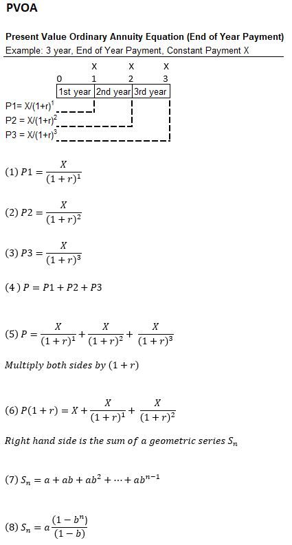
Present Value Ordinary Annuity (PVOA)
An Ordinary Annuity has End of Period payments. Ordinary Annuity Examples:
- Most loans like educational loans, auto loans, and home mortgages.
- Regular or recurring savings activities like with company 401k retirement accounts.
Example Use of PV Ordinary Annuity:
- How much to deposit today in order to receive a fixed amount at the end of each year (for a certain number of years) from an investment account.
The timeline below is a simple visual example of the general formula that follows (where P = P1 + P2 + P3).
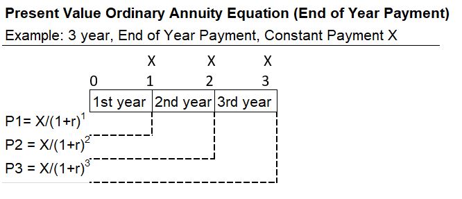
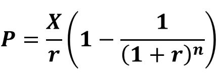
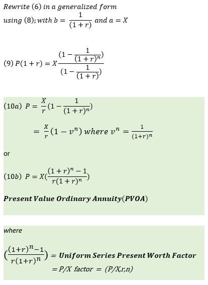
P = X/r(1-1/(1+r)n)
Refer to Appendix 6 for its derivation.
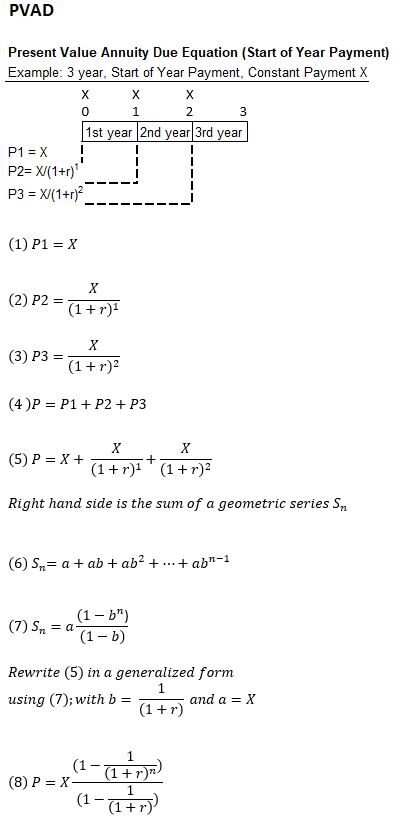
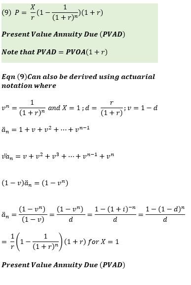
Present Value Annuity Due (PVAD)
An Annuity Due has Beginning of Period payments. Annuity Due Examples that are typically paid at beginning of period:
- Retirement income
- Tuition payments
- Rental payments
Example Use of PV Annuity Due:
- How much to deposit today in order to receive a fixed amount at the start of each year (for a certain number of years) from an investment account.
The timeline below is a simple visual example of the general formula that follows (where P = P1 + P2 + P3).
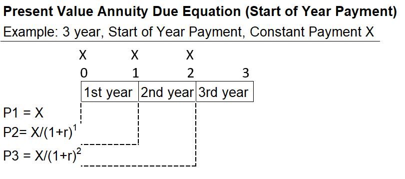
P = X/r(1-1/(1+r)n)(1+r)
Note that the value of an Annuity Due is always going to be larger than the value of an Ordinary Annuity.
Refer to Appendix 7 for its derivation.
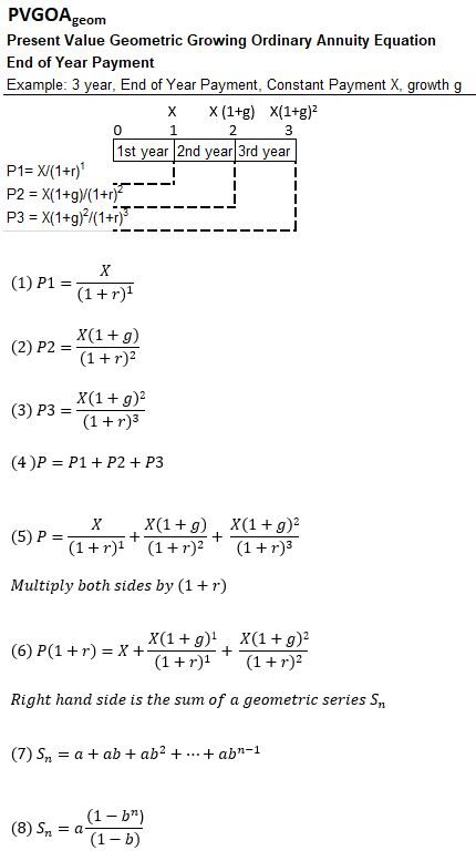
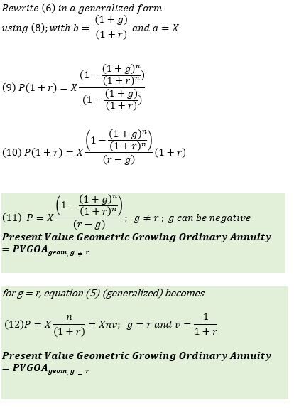
Present Value Geometrically Growing Ordinary Annuity (PVGOAgeom)
The timeline below is a simple visual example of the general formula that follows (where P = P1 + P2 + P3).
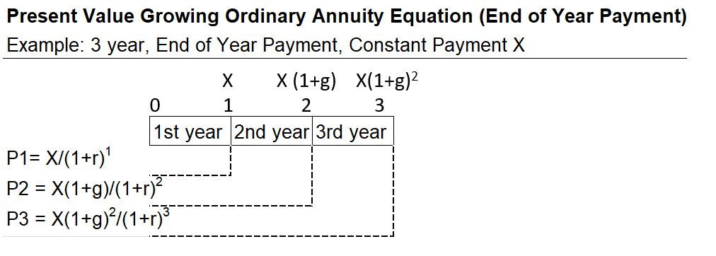
P = (X/(r-g))(1-(1+g)n/(1+r)n) ; g<r
Refer to Appendix 8 for its derivation.
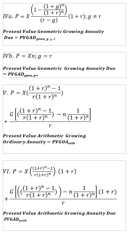
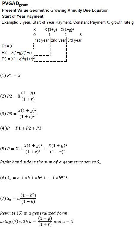
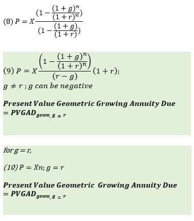
Present Value Geometrically Growing Annuity Due (PVGADgeom)
The timeline below is a simple visual example of the general formula that follows (where P = P1 + P2 + P3).
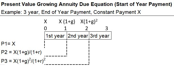
P = (X/(r-g))(1-(1+g)n/(1+r)n)(1+r) ; g<r
Note that the value of an Annuity Due is always going to be larger than the value of an Ordinary Annuity.
Refer to Appendix 9 for its derivation.
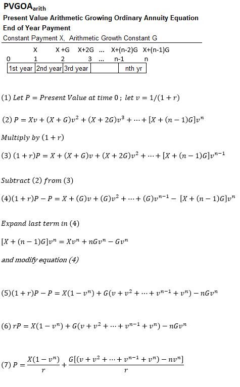
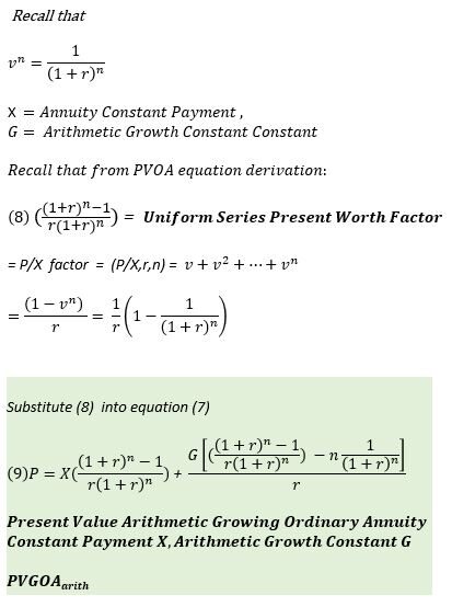
Present Value Arithmetically Growing Ordinary Annuity (PVGOAarith)
A PVGOAarith equation can be developed using a timeline like the one shown below.
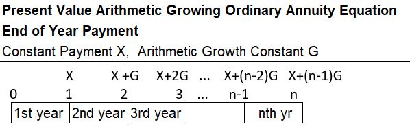
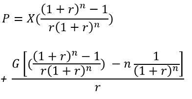
Refer to Appendix 10 for the equation and its derivation.
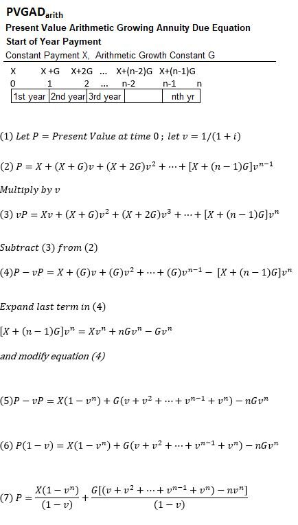
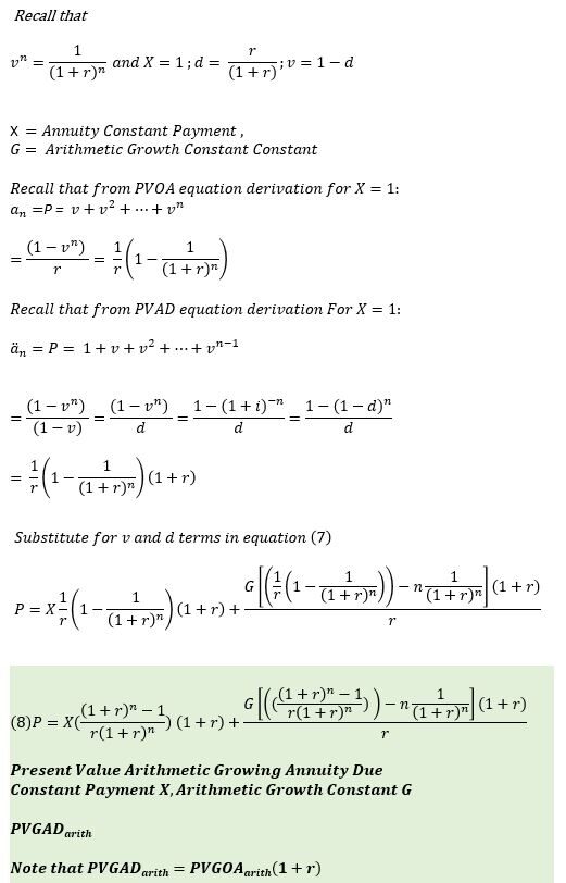
Present Value Arithmetically Growing Annuity Due (PVGADarith)
A PVGADarith equation can be developed using a timeline like the one shown below.
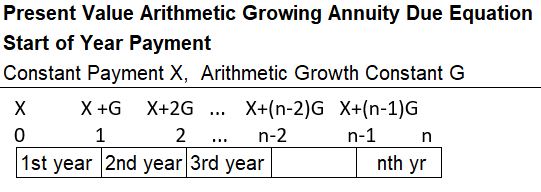
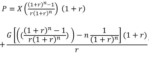
Refer to Appendix 11 for the equation and its derivation.
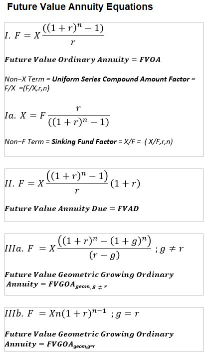
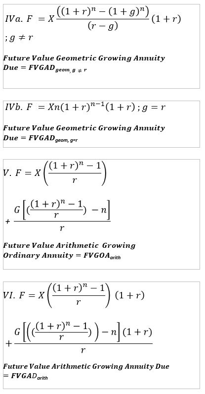
Future Value Annuity Formulas
Table 6 – Future Value Annuity Formulas
Variable Definitions
- F = Future Value
- X = Periodic Payment
- i = annual rate (expressed as fraction)
- c = compounding periods per year
- r = rate per period = i/c (expressed as fraction)
- Sn = sum of a finite geometric series
- a = geometric series start term
- b = geometric series common ratio
- y = number of years
- n = number of compounding periods =(c)(y)
- g = growth rate
- G = Arithmetic growth constant
Future Value Ordinary Annuity (FVOA)
An Ordinary Annuity has End of Period payments. Ordinary Annuity Examples:
- Most loans like educational loans, auto loans, and home mortgages.
- Regular or recurring savings activities like with company 401k retirement accounts.
Example Use of FV Ordinary Annuity:
- Compute the future value of periodic constant end of year contributions into an investment account.
The timeline below is a simple visual example of the general formula that follows (Where F = F1 + F2 + F3).
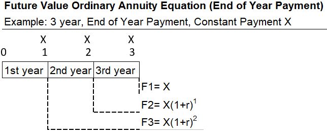
F = X((1+r)n – 1)/r
Refer to Appendix 12 for its derivation.
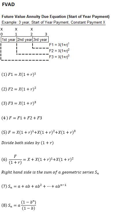
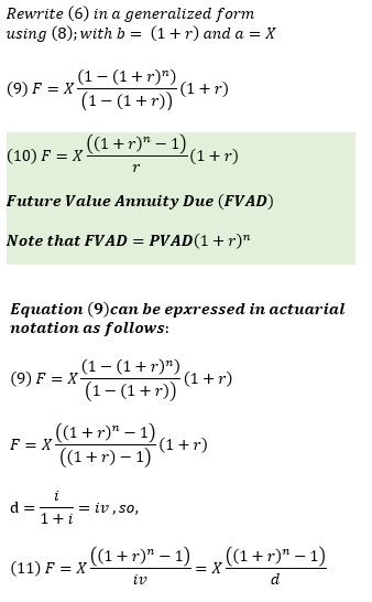
Future Value Annuity Due (FVAD)
An Annuity Due has Beginning of Period payments. Annuity Due Examples that are typically paid at beginning of period:
- Retirement income
- Tuition payments
- Rental payments
Example Use of FV Annuity Due:
- Compute the future value of periodic constant start of year contributions into an investment account.
The timeline below is a simple visual example of the general formula that follows (Where F = F1 + F2 + F3).
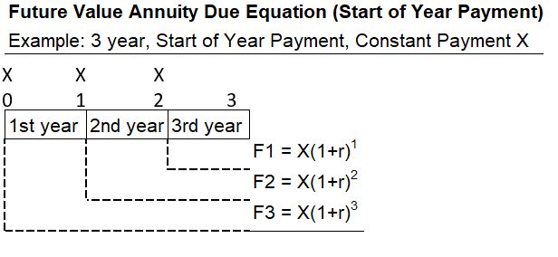
F = X((1+r)n – 1)(1+r)/r
Note that the value of an Annuity Due is always going to be larger than the value of an Ordinary Annuity.
Refer to Appendix 13 for its derivation.
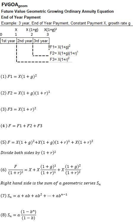
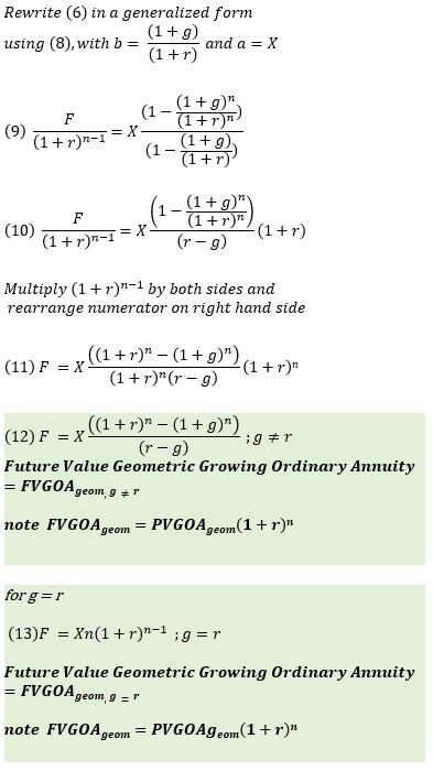
Future Value Geometric Growing Ordinary Annuity (FVGOAgeom)
The timeline below is a simple visual example of the general formula that follows (Where F = F1 + F2 + F3).
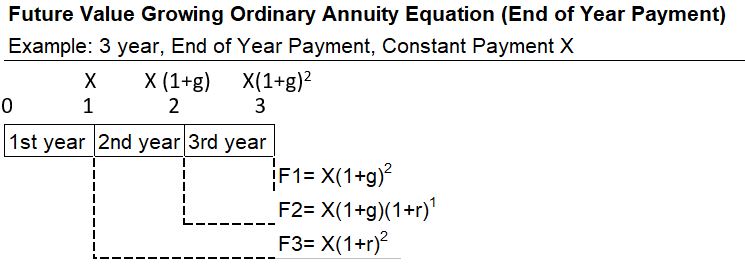
F = (X/(r-g))((1+r)n-(1+g)n) ; g<r
Refer to Appendix 14 for its derivation.
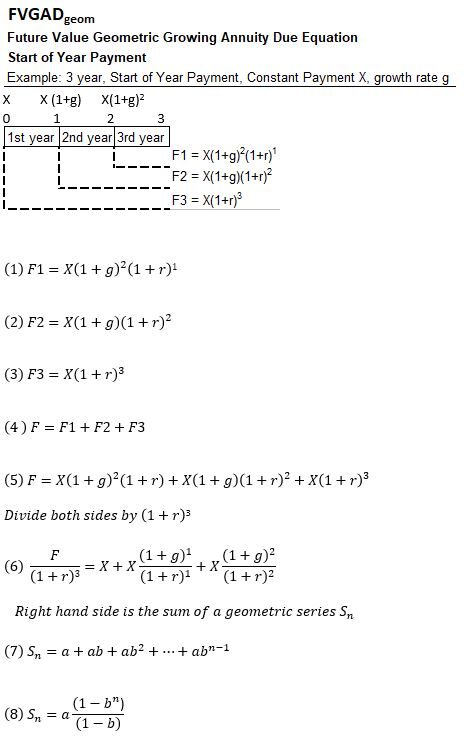
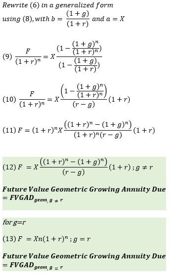
Future Value Geometric Growing Annuity Due
(FVGADgeom)
The timeline below is a simple visual example of the general formula that follows (Where F = F1 + F2 + F3).
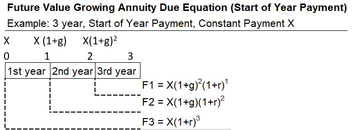
F = (X/(r-g))((1+r)n-(1+g)n)(1+r) ; g<r
Note that the value of an Annuity Due is always going to be larger than the value of an Ordinary Annuity.
Refer to Appendix 15 for its derivation.
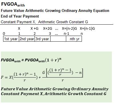
Future Value Arithmetically Growing Ordinary Annuity (FVGOAarith)
A FVGOAarith equation can be developed using a timeline like the one shown below.
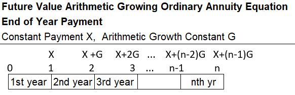
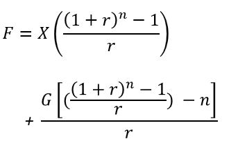
Refer to Appendix 16 for the equation and its derivation.
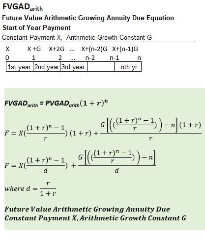
Future Value Arithmetically Growing Annuity Due (FVGADarith)
A FVGADarith equation can be developed using a timeline like the one shown below.
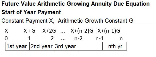
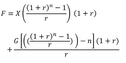
Refer to Appendix 17 for the equation and its derivation.
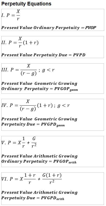
Perpetuity Formulas
Table 7 – Perpetuity Formulas
Variable Definitions
- F = Future Value
- X = Periodic Payment
- i = annual rate (expressed as fraction)
- c = compounding periods per year
- r = rate per period = i/c (expressed as fraction)
- y = number of years
- g = growth rate
- G = arithmetic growth constant
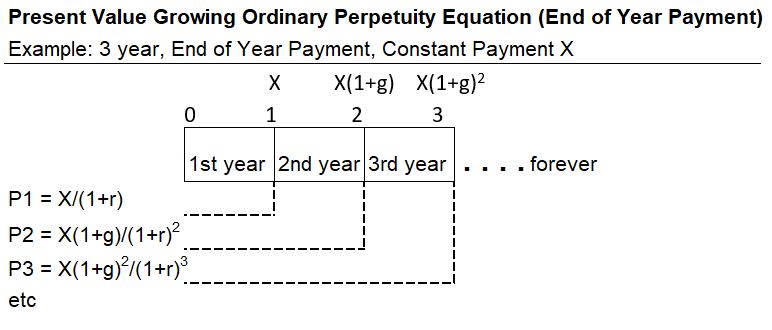
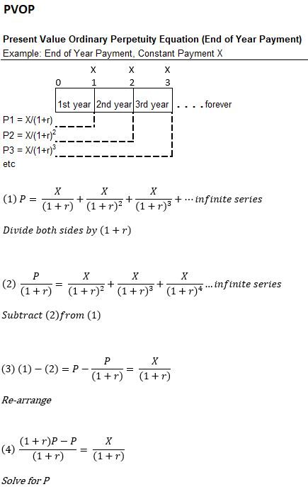
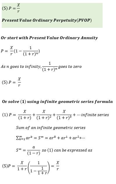
Present Value Ordinary Perpetuity (PVOP)
The timeline below is a simple visual example of the general formula that follows (Where P = P1 + +2 + P3).
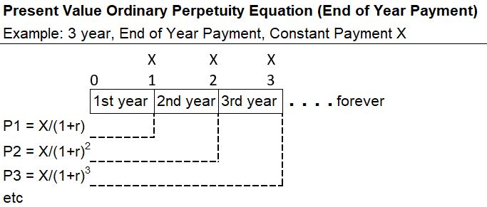
P = X/r
Refer to Appendix 18 for its derivation.
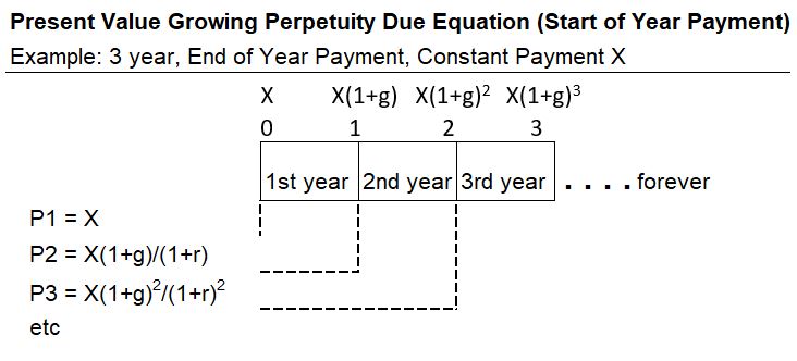
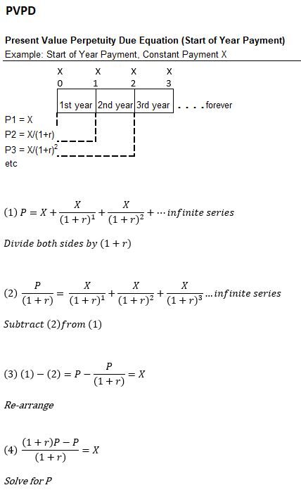
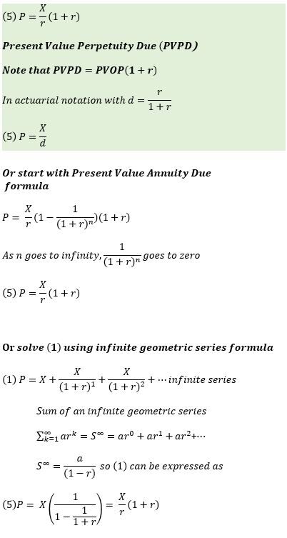
Present Value Perpetuity Due (PVPD)
The timeline below is a simple visual example of the general formula that follows (Where P = P1 + +2 + P3).
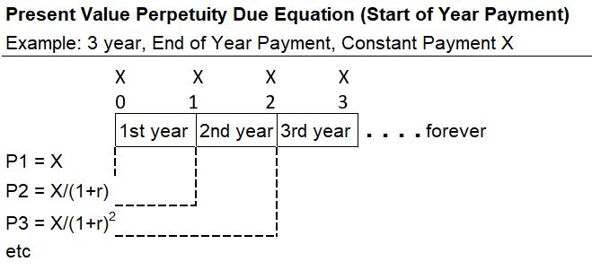
P = (1+r)X/r
Note that the Perpetuity Due will always be larger than the Ordinary Perpetuity.
Refer to Appendix 19 for its derivation.
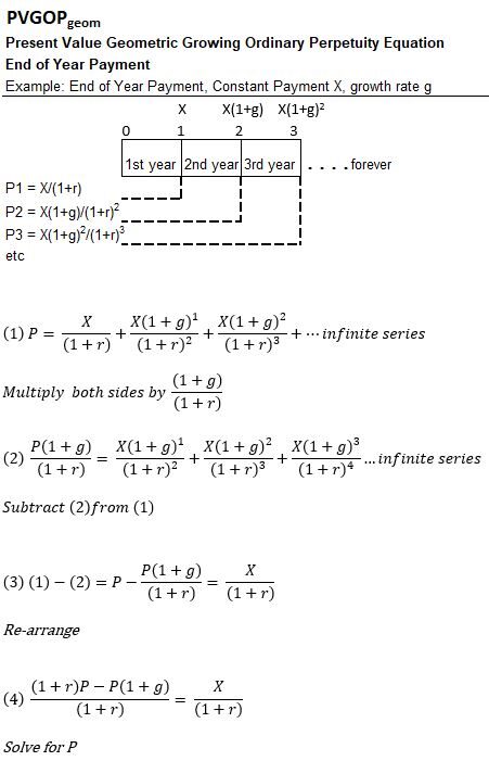
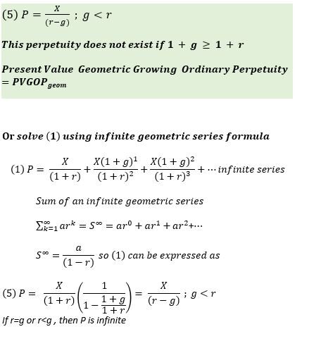
Present Value Geometric Growing Ordinary Perpetuity
(PVGOPgeom)
The timeline below is a simple visual example of the general formula that follows (Where P = P1 + +2 + P3).
P = X/(r-g) ; g<r
Refer to Appendix 20 for its derivation.
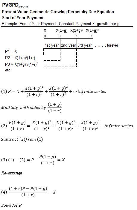
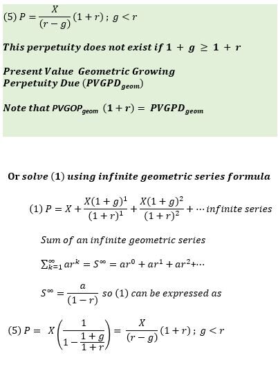
Present Value Geometrically Growing Perpetuity Due (PVGPDgeom)
The timeline below is a simple visual example of the general formula that follows (Where P = P1 + +2 + P3).
P = (1+r)X/(r-g) ; g<r
Note that the Perpetuity Due will always be larger than the Ordinary Perpetuity.
Refer to Appendix 21 for its derivation.
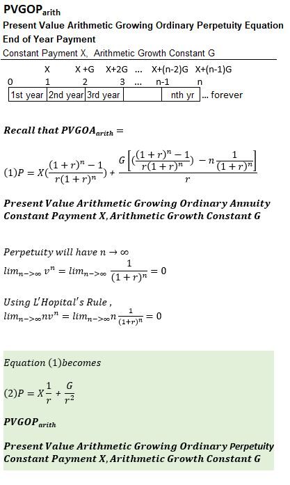
Present Value Arithmetically Growing Ordinary Perpetuity (PVGOParith)
A PVGOParith equation can be developed using a timeline like the one shown below.
Refer to Appendix 22 for the equation and its derivation.
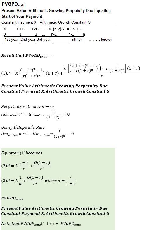
Present Value Arithmetically Growing Perpetuity Due (PVGPDarith)
A PVGPDarith equation can be developed using a timeline like the one shown below.
Refer to Appendix 23 for the equation and its derivation.
TVM Calculations Using a Financial Calculator
Your financial calculator can do single cash flow and Annuity (equal value and equal period cash flow) discounting and compounding calculations.
It can also do NPV calculations.
Single Cash Flow and Annuity Calculations
The 5 main keys used for these kinds of calculations on your financial calculator will look something like the below (they look exactly like this on my HP 12c calculator).

- y = number of years
- c = number of compounding periods per year
- i = rate per compounding period = (yearly rate)/c ; (see Note 1)
- n = number of compounding periods per year = (c)(y) (See Note 2)
- PV = Present Value
- FV = Future Value
- PMT = constant Annuity payments; BEG or END (See Note 3)
Note 1: Regarding i
- The HP 12c calculator key [i] is equivalent to the “r” that I have defined throughout this post.
- Just remember, when you enter the rate in any calculator or excel function you are always entering in the rate per compounding period.
Note 2: Regarding n
Note 3: Regarding PMT
- these are the secondary (blue colored typically) “END” or “BEG” keys.
- “END” is the default value.
Solving for a Particular Variable
Loan Calculations
Loans (debt repayments) are typically Ordinary Annuity type calculations.
Your financial calculator has a few additional keys to help you do these kinds of calculations.
Example: You take out a $200,000 home loan (30 year fixed; interest rate of 3%; monthly mortgage payments). What is the monthly mortgage payment and how much interest will have been paid after 5 payments?
- Key entries on the HP 12c: n = 30×12=360, PV=$200,000,i = 3/12=.25,FV=0.
- Pressing the PMT key gives – $843.21 = the monthly mortgage payment.
- Pressing “360 f Amort” gives -103,554.9 the total interest paid and
- Pressing the R↓ key gives -200,000, the principal paid.
(DCF) Discounted Cash Flow (NPV) Calculations
- We refer to uneven cash flows below.
- Don’t confuse this with uneven (or unequal cash flow intervals).
- The HP 12c always assumes equal intervals between cash flows.
- [CFo]: Time zero (current) cash flow amount (see Note 4)
- [CFj]: After time zero cash flow amounts for the jth period (see Note 5)
- [Nj]: A multiplier for equal cash flows (e.g. if you had 4 cash flows of 100, then you enter 10 with CFj, then with Nj you would indicate you want this repeated 4 times).
Note 5: Assumes end of period cash flow.
- an investment or a capital expense in time zero would be entered as a negative value and
- cash flows in future years would be entered as positive values.
- The required rate, the discount rate, is entered using the [i] key previously noted.
- The NPV is calculated using the [NPV] button, which is a secondary (orange) key on the HP 12c.
- Alternatively, the Internal Rate of Return can be computed with the [IRR] button which is also a secondary (orange) key on the HP 12c.
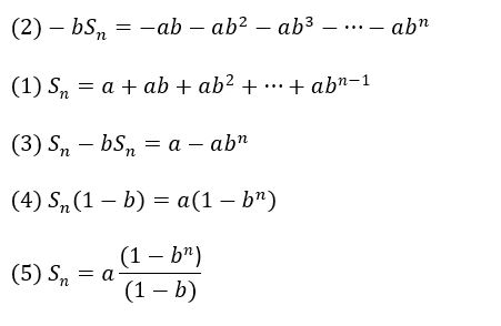
Appendix 2 – Sum of a Finite Geometric Series
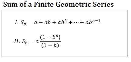
The equation for a finite geometric series summation is useful in the derivation of the annuity equations.
A Geometric Series can be expressed as,
Sn = a + ab + ab2 +…+abn-1
Where,
- Sn = sum of first n terms
- a = first term
- b = common ratio
- n = number of terms
A finite form of this can be expressed as,
Sn = a(1-bn)/(1-b)
Finite Summation Geometric Series
See a derivation of this equation below.
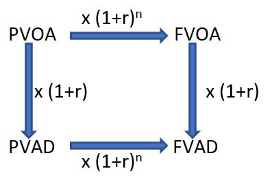
Appendix 4 – Annuity Equation Conversion factors
An Ordinary Annuity equation can be converted to its Annuity Due form by multiplying it by (1+r) where r is the interest rate.
A Present Value Annuity equation can be converted to it Future Value form by multiplying it by (1+r)n
Appendix 5 – Discount Factor v, Effective Rate of Discount Factor d, and some useful Limit relationships.
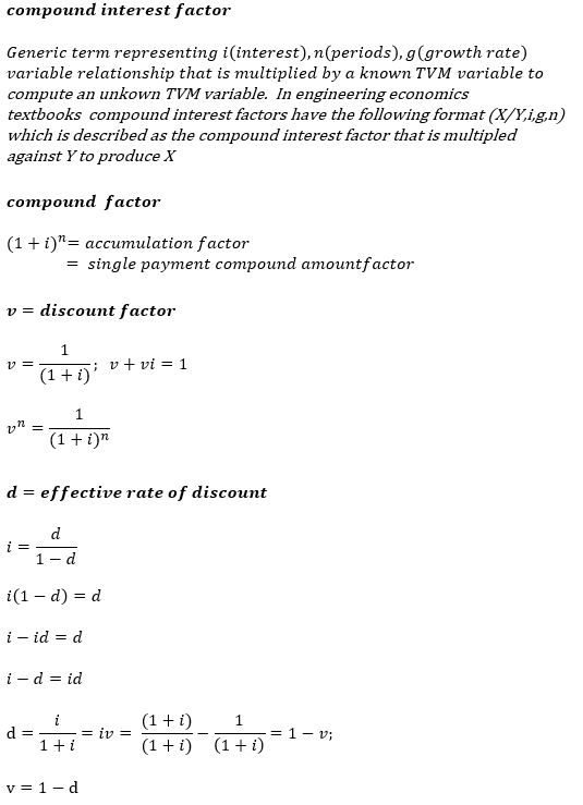
Compound(ing) Factor, Discount Factor v, and Effective Rate of Discount Factor d
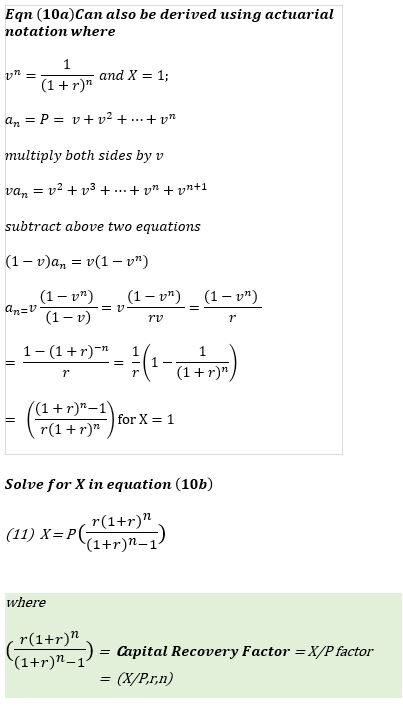
In actuarial texts, annuities are often expressed using variables v and d. The Discount Factor = v = 1/(1+r) where r is interest rate. The Effective Rate of Discount Factor = d = r/(1+r). See the picture below for various ways these can be expressed.
A Compound Interest Factor is the generic term for the mathematical expression [consisting of r, n, and/or arithmetic or geometric growth rates] that is multiplied against a given variable to compute the desired variable. For example to compute the Present Value of an Ordinary Annuity , the Constant Payment can be multiplied against a compound interest factor called the Uniform Series Present Worth Factor. Compound interest factors are often tabulated in textbooks for easy lookup.
Useful Limits and L’Hopital’s Rule
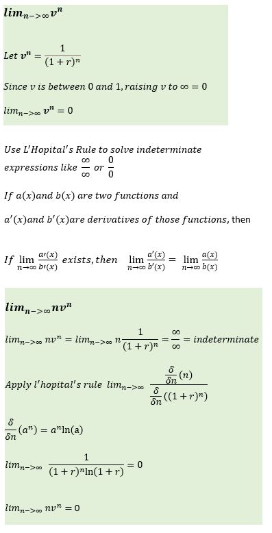
The limitn→∞1/(1+r)n is useful (= 0) when deriving perpetuity forms of the annuity equations.
Applying L’Hopital’s rule to find a solution to the limit of indeterminate values (e.g. limitn→∞n/(1+r)n which also equals 0) will also be useful when deriving perpetuity forms of annuity equations.
Appendix 6 – Present Value Ordinary Annuity (PVOA)
Annuity payments are constant period payments.
Consider a timeline where constant annuity payments X are made at the end of years 1, 2 ,3 etc.
This kind of annuity is known as an Ordinary Annuity. We want to compute the present value of these payments.
- P = Present Value of all payments
- X = constant payment
- r = interest rate per compounding period
- n = number of compounding periods (note: n = number of terms in the Sn equation)
- P1, P2, P3: Present Values X from end of years 1,2,3 etc.
We can discount these three payments to the present and then adjust the equation to arrive at,
P = X/r ( 1 – 1/(1+r)n )
Present Value Ordinary Annuity (PVOA)
See a full derivation below where we develop and generalize the PVOA equation starting with a simple 3 year timeline.
Appendix 7 – Present Value Annuity Due (PVAD)
Annuity payments are constant period payments. Consider constant annuity payments X starting now (time 0, start of year 1), with additional payments at the start of year 2 and 3 etc. (at 1 and 2).
This kind of annuity is known as an Annuity Due. We want to compute the present value of these payments.
- P = Present Value of all payments
- X = constant payment
- r = interest rate per compounding period
- n = number of compounding periods (note: n = number of terms in the Sn equation)
- P1, P2, P3: Present Values X from start of years 1,2,3 etc.
We can discount these three payments to the present and then adjust the equation to arrive at,
P = X/r ( 1 – 1/(1+r)n ) (1+r)
Present Value Annuity Due (PVAD)
Note that the Present Value Annuity Due = (Present Value Ordinary Annuity)(1+r)
See a full derivation below where we develop and generalize the PVAD equation starting with a simple 3 year timeline.
Appendix 8 – Present Value Geometric Growing Ordinary Annuity (PVGOAgeom)
Annuity payments are constant period payments. Consider geometric growing annuity payments X, X(1+g), X(1+g)2 etc. starting at end of years 1, 2, 3, etc. respectively.
This kind of annuity is known as an Geometric (exponential) Growing Ordinary Annuity. We want to compute the present value of these payments.
- X = constant payment
- g = constant growth rate of X
- r = interest rate per compounding period
- n = number of compounding periods (note: n = number of terms in the Sn equation)
- P1, P2, P3: Present Values of X, X(1+g), and X(1+g)2 etc. from end of years 1,2,3 etc.
We can discount these payments to the present and arrive at,
P = ( X/(r-g) )( 1-(1+g)n/ (1+r)n ) ; g ≠ r
Present Value Geometric Growing Ordinary Annuity PVGOAgeom
See a full derivation below where we develop and generalize the PVGOAgeom equation starting with a simple 3 year timeline.
Appendix 9 – Present Value Geometric Growing Annuity Due (PVGADgeom)
Annuity payments are constant period payments. Consider geometric growing annuity payments X, X(1+g), X(1+g)2 etc. starting at the start of years 1, 2, 3, etc. respectively.
This kind of annuity is known as a Geometric Growing Annuity Due. We want to compute the present value of these payments.
- P = Present Value of all payments
- X = constant payment
- g = constant growth rate of X
- r = interest rate per compounding period
- n = number of compounding periods (note: n = number of terms in the Sn equation)
- P1, P2, P3: Present Values X, X(1+g), and X(1+g)2 etc. from start of years 1,2,3 etc.
We can discount these payments to the present and then adjust the equation to arrive at,
P = ( X/(r-g) )( 1-(1+g)n / (1+r)n )(1+r) ; g≠r
Present Value Geometric Growing Annuity Due PVGADgeom
Note that Present Value Geometric Growing Annuity Due = (Present Value Geometric Growing Ordinary Annuity)(1+r)
See a full derivation below where we develop and generalize the PVGADgeom equation starting with a simple 3 year timeline.
Appendix 10 – Present Value Arithmetic Growing Ordinary Annuity (PVGOAarith )
An arithmetically growing annuity , grows linearly at a constant value G. A PVGOAarith begins with a constant X paid at the end of year 1, followed by X+G, X+2G, etc.. at the end of subsequent years.
See the timeline and details below for a derivation of the PVGOAarith equation.
Appendix 11 – Present Value Arithmetic Growing Annuity Due (PVGADarith)
An arithmetically growing annuity , grows linearly at a constant value G. A PVGADarith begins with a constant X paid at the beginning of year 1, followed by X+G, X+2G, etc. at the end of subsequent years.
See the timeline and details below for a derivation of the PVGADarith equation. Note that PVGADarith = PVGOAarith(1+r).
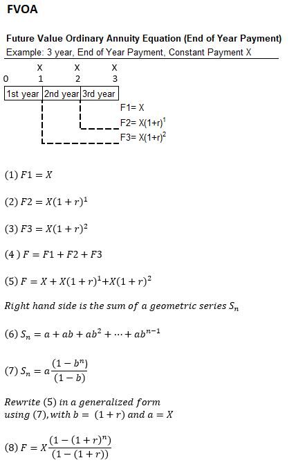
Appendix 12 – Future Value Ordinary Annuity (FVOA)
Annuity payments are constant period payments. Consider an annuity, known as an Ordinary Annuity, that pays out X at the end of Years 1, 2, 3, etc.
We want to compute the future value of these payments.
- F = Future Value of all payments
- X = Constant Payment
- r = interest rate per compounding period
- F1, F2, F3: Future Values of X from end of years 1, 2, 3.
- n = number of compounding periods
We can compound these payments to the future and come up with the following equation.
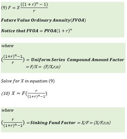
F = X ( (1+r)n – 1) /r
Future Value Ordinary Annuity (FVOA)
See a full derivation below where we develop and generalize the FVOA equation starting with a simple 3 year timeline.
Appendix 13 – Future Value Annuity Due (FVAD)
Consider constant annuity payments X starting now (time 0, start of year 1), with additional payments at the start of year 2 and 3 (at 1 and 2) etc. This kind of annuity is known as an Annuity Due. We want to compute the future value of these payments.
- F = Future Value of all payments
- X = Constant Payment
- r = interest rate per compounding period
- n= number of compounding periods
- F1, F2, F3: Future Values of X from the start of years 1, 2, 3 etc.
F = X ( (1+r)n – 1)(1+r) / r
Future Value Annuity Due (FVAD).
Note that Future Value Annuity Due = (Future Value Ordinary Annuity)(1+r)
See a full derivation below where we develop and generalize the FVAD equation starting with a simple 3 year timeline.
Appendix 14 – Future Value Geometric Growing Ordinary Annuity (FVGOAgeom)
Annuity payments are constant period payments. Consider growing annuity payments X, X(1+g), and X(1+g)2 etc. starting at end of years 1, 2, 3 etc. respectively.
This kind of annuity is known as a Geometric Growing Ordinary Annuity. We want to compute the future value of these payments.
- F = Future Value of all payments
- X = constant payment
- g = constant growth rate of X
- r = interest rate per compounding period
- n = number of compounding periods (note: n = number of terms in the Sn equation)
- F1, F2, F3: Future Values X, X(1+g), and X(1+g)2 etc. from end of years 1,2,3 etc.
We can compound these payments to the future and come up with the following equation.
F = (X/(r-g))((1+r)n-(1+g)n) ; g≠r
Future Value Geometric Growing Ordinary Annuity FVGOAgeom
See a full derivation below where we develop and generalize the FVGOAgeom equation starting with a simple 3 year timeline.
Appendix 15 – Future Value Geometric Growing Annuity Due (FVGADgeom)
Annuity payments are constant period payments. Consider geometric growing annuity payments X, X(1+g), and X(1+g)2 etc. starting at the start of years 1, 2, 3 etc. respectively.
This kind of annuity is known as an Geometric Growing Annuity Due. We want to compute the future value of these payments.
- F = Future Value of all payments
- X = constant payment
- g = constant growth rate of X
- r = interest rate per compounding period
- n = number of compounding periods (note: n = number of terms in the Sn equation)
- F1, F2, F3 etc.: Future Values X, X(1+g), and X(1+g)2 etc. from start of years 1,2,3 etc.
We can compound these payments to the future and come up with the following equation.
F = ( X/(r-g) )( (1+r)n-(1+g)n )(1+r) ; g≠r
Future Value Geometric Growing Annuity Due FVGADgeom
Note that Future Value Geometric Growing Annuity Due = (Future Value Geometric Growing Ordinary Annuity)(1+r)
See a full derivation below where we develop and generalize the FVGADgeom equation starting with a simple 3 year timeline.
Appendix 16 – Future Value Arithmetic Growing Ordinary Annuity (FVGOAarith)
An arithmetically growing annuity , grows linearly at a constant value G. A FVGOAarith begins with a constant X paid at the end of year 1, followed by X+G, X+2G, etc.. at the end of subsequent years.
See the timeline and details below for a derivation of the FVGOAarith equation.
Appendix 17 – Future Value Arithmetic Growing Annuity Due (FVGADarith)
An arithmetically growing annuity , grows linearly at a constant value G. A FVGADarith begins with a constant X paid at the beginning of year 1, followed by X+G, X+2G, etc. at the end of subsequent years.
See the timeline and details below for a derivation of the FVGADarith equation. Note that FVGADarith = FVGOAarith(1+r).
Appendix 18 – Present Value Ordinary Perpetuity (PVOP)
A perpetuity is an annuity that goes on forever. Consider an Ordinary Perpetuity that pays out X at the end of each year.
Let’s derive the Present Value Ordinary Perpetuity equation.
- P = Present Value of all payments
- X = constant payment
- r = interest rate per compounding period
- P1, P2, P3 etc.: Present Values X from end of years 1,2,3 etc.
After discounting the terms and doing a few simple mathematical manipulations to the resultant infinite series we get,
P = X/r
Present Value Ordinary Perpetuity (PVOP)
See a full derivation below:
Appendix 19 – Present Value Perpetuity Due (PVPD)
A perpetuity is an annuity that goes on forever. Consider a Perpetuity Due that pays out X at the start of each year.
Let’s derive the Present Value Perpetuity Due equation.
- P = Present Value of all payments
- X = constant payment
- r = interest rate per compounding period
- P1, P2, P3 etc.: Present Values X from start of years 1,2,3 etc.
After discounting the terms and doing a few simple mathematical manipulations to the resultant infinite series we get,
P = (1+r)X/r
Present Value Perpetuity Due (PVPD)
Note that the Present Value Perpetuity Due = (Present Value Ordinary Perpetuity)(1+r)
See a full derivation below:
Appendix 20 – Present Value Geometrically Growing Ordinary Perpetuity (PVGOPgeom)
Geometric Growing Perpetuity payments are constant period payments that grow exponentially and go on forever.
Consider geometrically growing payments X, X(1+g), and X(1+g)2 etc. starting at end of years 1, 2, etc. respectively (a Geometric Growing Ordinary Perpetuity).
We want to compute the present value of these payments.
- P = Present Value of all payments
- X = constant payment
- g = constant growth rate of X
- r = interest rate per compounding period
- P1, P2, P3 etc.: Present Values X/(1+r), X(1+g)/(1+r)2, and X(1+g)2 /(1+r)3 etc. from end of years 1,2,3 etc.
After discounting the terms and doing a few simple mathematical manipulations to the resultant infinite series we get,
P = X/(r-g) ; g<r
Present Value Growing Ordinary Perpetuity PVGOPgeom
See a full derivation below:
Appendix 21 – Present Value Geometrically Growing Perpetuity Due (PVGPDgeom)
Perpetuity payments are annuities that go on forever. Consider geometrically growing annuity payments X, X(1+g), and X(1+g)2 etc.. starting at the start of years 1, 2, 3 etc. respectively.
This kind of annuity is known as a Geometrically Growing Perpetuity Due. We want to compute the present value of these payments.
- P = Present Value of all payments
- X = constant payment
- g = constant growth rate of X
- r = interest rate per compounding period
- P1, P2, P3: Present Values X, X(1+g)/(1+r), and X(1+g)2 /(1+r)2 from start of years 1,2, etc.
After discounting the terms and doing a few simple mathematical manipulations to the resultant infinite series we get,
P = (1+r)X/(r-g) ; g<r
Present Value Growing Perpetuity Due PVGPDgeom
Note that Present Value Geometrically Growing Perpetuity Due = (Present Value Geometrically Growing Ordinary Perpetuity)(1+r)
See a full derivation below:
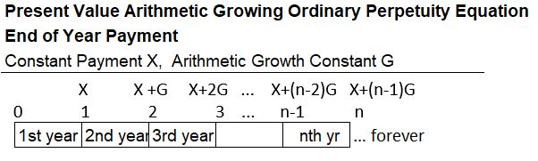
Appendix 22 – Present Value Arithmetically Growing Ordinary Perpetuity (PVGOParith)
Arithmetically Growing Perpetuity payments are constant period payments that grow linearly and go on forever.
Consider arithmetically growing payments X, X+G, X+2G etc. starting at end of years 1, 2, 3 etc. respectively (an Arithmetically Growing Ordinary Perpetuity).
We want to compute the present value of these payments.
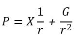
We can derive this by starting with the equation for a PVGOAarith and letting n →∞.
P = X/r + G/r2
Present Value Arithmetically Growing Ordinary Perpetuity PVGOParith
See a full derivation below:
Appendix 23 – Present Value Arithmetically Growing Perpetuity Due (PVGPDarith)
Arithmetically Growing Perpetuity payments are payments that grow linearly and go on forever. Consider arithmetically growing annuity payments X, X+G, and X+2G etc. starting at the start of years 1, 2, 3 etc. respectively. Both X and G are constants. We want to compute the present value of these payments.
We can derive this by starting with the equation for a PVGADarith and letting n →∞.
P = X(1+r)/r + G(1+r)/r2
Present Value Growing Perpetuity Due PVGPDarith
Note that PVGPDarith = PVGOParith(1+r)
See a full derivation below:
Appendix 24 – Continuous Compounding Formula Derivation
Let’s derive the equation for continuous (infinite) compounding.
Consider the expression (1+1/c)c
The table below shows that as c increases, the expression approaches a value called Euler’s Number, e.
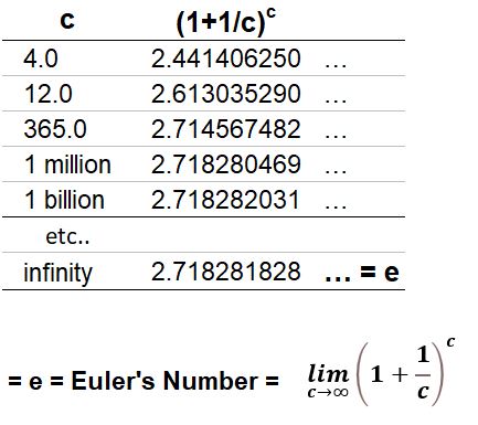
Euler’s Number is an amazing number, and it will figure into our infinite compounding derivation, but first let’s take a little diversion.
A Diversion
Euler’s number is a non-terminating number (endless) and it can’t be expressed as a fraction (i.e. it’s an irrational number).
Its description as “e” was used by Swiss mathematician Leonhard Euler (pronounced “Oiler”) in ~1731.
So Euler coined the constant e and popularized it, but
- the constant was used by British Mathematician John Napier in ~1614 and
- was first discretely described by Jacob Bernoulli (another famous Swiss mathematician!). (Source: Wikipedia).
Some cool facts that are not really relevant to our derivation , but , need to be mentioned, because you should be amazed:
- Euler’s can be defined a few other ways. Here is one of those:
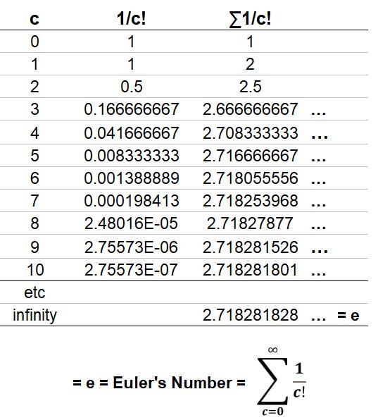
- c! = c”factorial” meaning: For c>0, c! = 1×2×3×4×…×c For n=0; 0! = 1
- Another non-terminating and irrational number is Pi (π = 3.14159…)
- And, for those who argue there is order in the universe, e and π are related through the Euler Identity.
- The Euler Identity: eiπ +1 = 0
- You really should watch Sal Khan’s (khanacademy) derivation of the Euler Identity: Start with his video on the imaginary unit i and then view his video on Euler’s formula and Euler’s Identity.
Ok back to the task at hand.
Continuous (Infinite) Compounding Equation Derivation
Refer to the great tutorials by Sal Khan on how to derive the infinite compounding formula.
Remember the Compound Interest Formula for a Single Cash Flow where,
- F = P(1+r)n = P(1+i/c)cy
- F = Future Value, P = Present Value,
- i = yearly interest rate (sometimes called the stated rate)
- c = number of compounding periods per year
- r = interest rate per compounding period = i/c
- y = number of years
- n = total number of compounding periods = (c)(y)
Start with our compounding formula.
(1) F = P(1+i/c)cy
Assume c is going to infinity. Then
(2) F = lim(c→∞) [ P(1+i/c)cy ]
Now we want to substitute and let x = c/i. So c = xi and i/c = 1/x.
Substitute for c and i/c in equation (2). We get,
(3) F = lim(x→∞) [ P(1+1/x)xiy ] which equals
(4) F = P [ lim(x→∞) (1+1/x)x ] iy . The limit expression in this equation we know is equal to e, Euler’s number, so,
(5) F = P e iy = Equation for Continuous Compounding
Very nice.