Gauss's Law of Electricity (of the Electric Field)

Menu (linked Index)

Gauss’s Law of Electricity (of the Electric Field)

Last Update: August 22, 2025

Introduction
Water Flow Analogy for Electric Flux
General Form of Uniform Electric Flux through A Flat Surface
Flux of a Non-Uniform Electric Field through an Irregular Surface
Area Vectors
Electric Flux Definition Using the Area Vector
Gauss’s Law of Electricity
Appendix 1: Coulomb’s Law, Electric Force, and Electric Field
Appendix 2: E Flux is Constant Regardless of Position of Enclosed Charge
Appendix 3: Converting the Integral Form of Gauss’s Law of Electricity into Differential Form

Introduction

In this post I describe electric flux and Gauss’s Law of Electricity.

Gauss’s Law of Electricity is one of the four famous so called Maxwell Equations of electromagnetism.

Using simple illustrations, I built up from basic concepts to the general form of the equation.

This post is mostly a faithful rendering of Mahesh Shenoy’s (Khanacademy) videos on the subject.

They are really good and you should watch them.

Other good references:

To see the other famous Maxwell Equations see my Post: From Maxwell’s Equations to The Wave Equation
To study up on vectors see my post: Vector Math
To study up on vector operators, see my post: Field Operators: Grad, Div, and Curl
Introduction to Gauss’ Law | Physics with Professor Matt Anderson | M17-07
Intro to Electric Flux & Gauss’s Law – PhysicsOMG

Return to Menu

Water Flow Analogy for Electric Flux

Consider water flowing in a duct where it passes a perpendicular cross sectional area as shown in Graph_1.

Graph_1: Volumetric Flow Analogy to Electric Flux

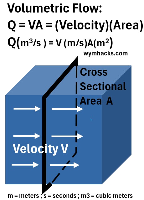
If the water is flowing at a certain velocity V and it crosses this area A, then

the volumetric flow rate will be equal to the product of V and A and
will have units of volume per time.

In Graph_1, the volumetric flow rate Q = (V)(A) has units of cubic meters per second (m³/s).

Analogous to water flow, the Electric Flux, sometimes symbolized with Φ (Phi), is a measure of how much an electric field passes through a specific surface.

Graph_2: Electric Flux Through a Flat Perpendicular Surface

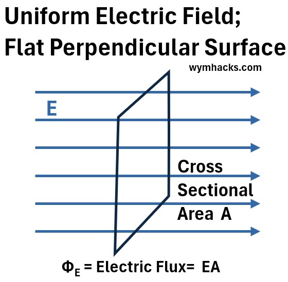
Φ = Electric Flux = (E)(A) for Uniform E and Flat Surface Perpendicular to E

where,

Φ = Electric Flux
- has units of (Newton/Coulomb)m² = (N/C)m²
A (in m²) = Perpendicular cross sectional area the electric field passes through
E = The electric field (a vector field).
- has units of Newton/Coulomb = N/C

An increasing/decreasing E or A will result in an increasing/decreasing electric flux.

Return to Menu

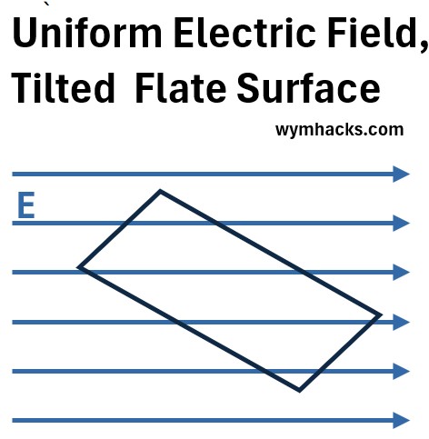
General Form of Uniform Electric Flux through a Flat Surface

Now consider a uniform field E going through a tilted non-perpendicular flat surface.

Assuming the same E field in Graph_2 and Graph_3, you can see that less of the Electric field passes through the tilted surface.

Graph_3: Electric Flux through a Tilted Flat Surface

Graph_4 shows a side view of the E Field Passing through various orientations of the flat surface.

Graph_4: Electric Flux Drops as Surface Area Tilts from the Vertical

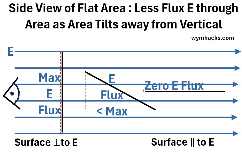
Less “E” travels through the surface area as the area tilts towards the horizontal.

As noted by the red dotted lines, it is this effective area, that affects the flux.
The effective area is the component of the surface that is perpendicular to the E field vectors.

So, lets develop a more general form of the flux for a uniform field through a flat surface.

Consider Graph_5 below where E passes through surface A, and where the perpendicular component of A is A_p.

Graph_5: Side View Electric Flux through Flat Flow Area

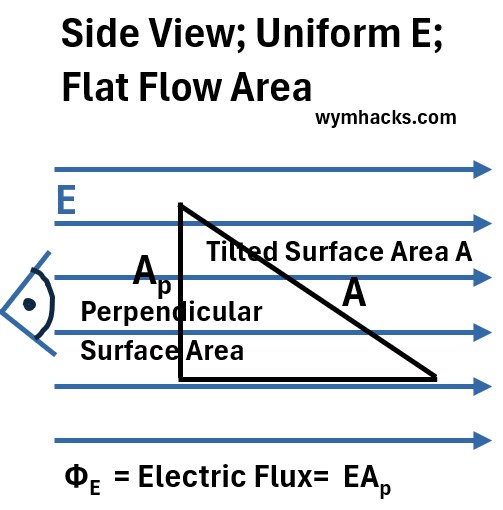
Φ = Electric Flux = (E)(Ap) for Uniform E and Flat Surface

where,

Φ = Electric Flux (units: (N/C)m2)
A_p (units: m²) = Perpendicular component of A that the electric field passes through
E = The electric field (units: N/C)

Return to Menu

Flux Of a Non-Uniform Electric Field through an Irregular Surface

Ok, now lets continue generalizing the electric flux equation and assume the E field is not uniform and it is going through a non-uniform surface.

Graph_6: Electric Flux for Non-Uniform E through An Irregular Surface

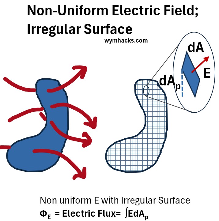
This is where the calculus of integration becomes very useful.

Partition the surface up into infinitesimally small and now flat surfaces.
Take one of these surfaces and label its surface area as dA, with the d meaning infinitely small.
Using the concept as before we can also label the perpendicular component as dA_p

We can now use the mathematics of integrals (summations of infinitesimals) to come up with a more general equation for the electric flux.

Φ = Electric Flux = ∫EdA_p for any E for any surface

where,

∫ is the integral which sums up all the infinitesimal products of E and dAp for all infinitesimal sections that make up the surface
Φ = Electric Flux (units: N/C)m2
dA_p (units: m²) = for an infinitesimally small surface, the Perpendicular component of A that the electric field passes through
E = The electric field (units: N/C) at that infinitesimally small surface

Unless we have simplifying assumptions, the E and the dA_p have to say inside the integral (they can be different for various small surfaces).

Well, we can do some more generalizing , but I have to introduce the concept of area vectors first.

Return to Menu

Area Vectors

Area vectors are a mathematical convention that are crucial for calculating electric flux .

The flux is found by taking the dot product of the field vector and the area vector, which mathematically accounts for the orientation.

Let’s remember what a dot product is first.

Vector Dot Product Geometric Definition

Given two vectors $a$ and $b$ in Euclidean space, their dot product is the product of their magnitudes and the cosine of the angle $θ$ between them:

where is the magnitude (length) of vector ,
and is the magnitude of vector .

Area Vectors

Take a look at Graph_7 as you read this section.

Graph_7: Area Vectors for Open and Closed Shapes

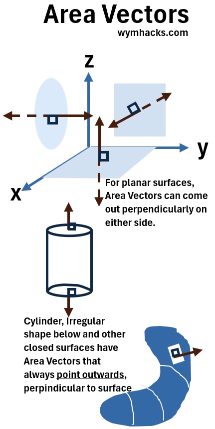
The arrows coming off at right angles in the drawing above are area vectors.
For open surfaces like the planar surfaces drawn in the xyz space, the direction of the arrow is arbitrary.
For closed surfaces, more of interest to us, the convection is always that the area vector points outwards (not inwards)
- As shown for the cylinder and the potato looking thing.
Area vectors represent the position of a surface in three dimensions.
Their magnitude is equal to the scalar area of the surface
- For a flat surface, the magnitude of the area vector is its area.
- For a curved surface, it’s defined by the sum of the magnitudes of infinitesimal area vectors.
An area vector’s direction is defined as being perpendicular (or normal) to that surface.
- For a closed surface (like a sphere), the convention is that the area vector points outward.
- For an open surface, the direction is arbitrary, but it must be chosen consistently for a given problem.

Ok, now, lets revisit our flux definition.

Return to Menu

Electric Flux Definition Using the Area Vector

Ok, lets redraw Graph_5 and incorporate the area vector concept.

Graph_8: Side View; Electric Flux for Uniform Field through Flat Surface with Area Vector

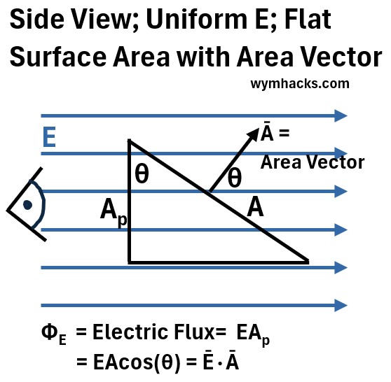
The area vector , shown as the arrow emanating from surface A represents the area of A and is perpendicular to A.

Note that in order to calculate A_pusing basic trigonometry, we need to know θ (because A_p= Acos(θ))

And , crucially, note that θ will always equal the angle the area vector makes with the E field vector.

So, this allows us to restate the electric flux for a uniform E and a flat surface as:

Φ = Electric Flux = (E)(Ap) =EAcos(θ) =Ē•Ā ; for Uniform E and Flat Surface

where,

Φ = Electric Flux (units: (N/C)m2)
A_p (units: m²) = Perpendicular component of A that the electric field passes through.
E = The electric field (units: N/C)
Ē•Ā = dot product of the electric field vector and the area vector.
θ = angle between area vector and E vector

We can follow the same logic we followed before for any E through any surface by using the integral of E times infinitesimal areas.

Φ = Electric Flux = ∫EdAcos(θ) =∫Ē•dĀ for any E for any surface

where, we now have a general expression for the electric flux through any surface.

Nice! But there are some other manipulations we can do to make the flux equation even more general.

Return to Menu

Gauss’s Law of Electricity

Ok, now, lets consider a spherical area (with radius R) around a central positive electric charge.

Flux E in a Sphere Containing a Central Charge

Graph_9: Electric Flux from a Sphere with Positive Charge at Center.

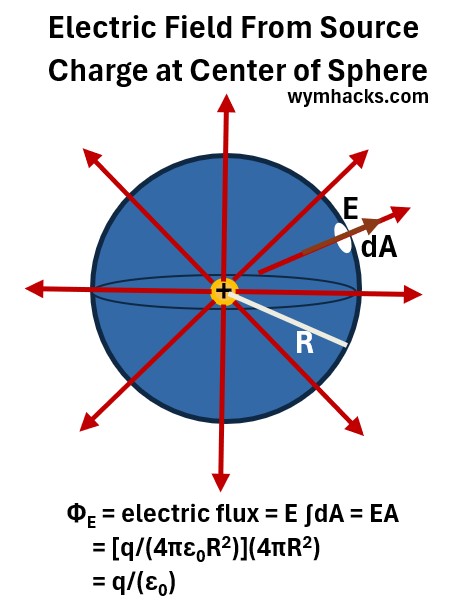
We want to calculate the electric flux for E through this sphere.

Let’s start with our general form of the electric flux equation:

Φ = Electric Flux =∫EdAp = ∫EdAcos(θ) =∫Ē•dĀ for any E for any surface and Flat Surface

For everywhere on the surface dA,

the surface is perpendicular to the radius R which is parallel to E.
So, θ = 0 and cos(0) = 1
and E is constant so

Φ = E ∫dA = EA

From Coulomb’s Law (see Appendix 1) we know that

E = F_e/q_2(test) = kq_1(source)/R²and
k = 1/(4πε₀)

Substituting into our flux equation we get,

Φ = [q/(4πε₀R²)](4πR²)

Φ = q/ε₀

Where q is (+) for a positive charge and q is (-) for a negative charge.

What Happens if we Adjust The Radius R?

Nothing. There is no R term in the spherical Flux equation.

Flux is independent of size due to inverse square law characteristic of Coulomb’s law.

What Happens if We Move The Charge Off Center in the Sphere?

Even though E and θ are no longer constant, the flux will remain the same (see Appendix 2 for the proof).

What Happens if We Have a Charge in some Non-Uniform Surface?

As long as the surface is closed, it doesnt matter. Flux is the same. The proof provided in Appendix 2 is independent of shape.

What Happens if We Have More Than One Charge Enclosed in the Area?

Just sum up the charges i.e. Φ = Σq/ε₀

What Happens if We Have Charges Outside the Surface?

Charges outside a closed surface do not contribute to the net electric flux through that surface.

So we began with a specific scenario of a Sphere but ended up with the most general form of the equation for the E flux.

∫Ē•dĀ = q_enclosed/ε₀ ; Gauss’s Law for Electricity ; Integral Form

Where q is the charge enclosed in the surface (any closed surface)
This equation is called Gauss’s Law for Electricity (or for the Electric Field)
It is the integral form of one of the four Maxwell Equations.

Differential Form of Gauss’s Law for Electricity

In my post From Maxwell’s Equations to The Wave Equation, I describe the differential form of Gauss’s Law for Electricity and the mathematical language behind it.

∇⋅E = ρ/ε₀ = 4πkρ ; Gauss’s Law for Electricity ; Differential Form

Variable Descriptions

∇⋅ = Divergence Operator where ∇ = nabla or del.
E = Electric Vector Field
ρ = charge density = charge/volume = q/V
ε₀= electric permittivity of free space
- It is a fundamental physical constant that represents the ability of a vacuum to permit electric field lines.
- ε_{0 =}8.854×10⁻¹² Farads per meter (F/m)
k = Coulomb’s Constant = electrostatic constant = 1/(4π ε₀) ≈8.99×10⁹N⋅m²/C²
μ₀ = magnetic permeability of free space = magnetic constant = 4π×10^-7 H/m (Henrys per meter).
- It is a fundamental physical constant that describes how a vacuum responds to a magnetic field.
c = 1/sqrt(μ₀ε₀) = speed of light = 299,792,458 m/s
π = pi = 3.1415..

Gauss’s Law for Electricity in Words

Gauss’s Law for electricity states that electric charges q give rise to electric fields E in a direction based on the sign of the electric charge.

From the differential form the law tells us:

a charge q (where ρ = charge/volume) creates an electric field E.
electric fields E act in a divergent way (∇⋅E) , meaning they are flowing outward or inward.
An electric charge acts as a source or sync for the electric field E.

From the integral form the law tells us:

The electric flux emanating from a close surface is equal to the charge enclosed by that surface.
The flux of a vector field is the amount of the field passing through the closed surface

Converting The Integral Form to the Differential Form

We can convert Gauss’s Law for Electricity from the integral form to the differential form by applying the Divergence Theorem.

See Appendix 3 for the details.

Return to Menu

Appendix 1: Coulomb’s Law , F_e, and E

Electrostatic Force

F_e = kq₁q₂/r²

F_e = electrostatic force
q₁, q₂ =The quantity of charge of objects 1 and 2
F is positive when q1 and q2 are of like charge and negative when q1 and q2 are of opposite charge.
r = distance between the charges.
Notice the inverse square relationship between force and distance.
k = 1/(4πε₀) = coulomb’s constant
ε₀ = electric constant = electric permittivity of free space (i.e. a vacuum)
ε₀ = 8.854e-12 C² / Nm² or can use units of “F/m” or “s⁴A²/(m³kg)”
k = 8.99e9 Nm²/C²
F = farad
1 F = 1 s⁴A²/(m²kg) where
A = ampere
1 A = 1 C/s
m = meters
kg = kilograms

In general Permittivity ε indicates how much a material resists the formation of an electric field within it.

A material with high permittivity will oppose the formation of an electric field more strongly
than a material with low permittivity.

ε₀is a measure of how dense of an electric field is “permitted” to form in response to electric charges (in a vacuum).

ε₀is a measure of how “permissive” the vacuum of space is to the formation of an electric field (which are generated by electric charges).
ε₀ tells you the relationship between the amount of charge and the strength of the electric field it creates in empty space.

Electrostatic Field E

E = F_e/q_2(test) = kq_1(source)/r²

E = magnitude of the electric field = electric field strength = Force/Charge
q₁ = source charge (produces the electric field) = q_s
q₂ = test charge (entering the electric field of q₁) = q_t
k = coulomb’s constant
SI units for E: Newtons/Coulomb = N/C
Other SI units for E = Nm/Cm = Volts/meter = V/m
N = newton
C = coulomb
V = voltage
M = meter

Return to Menu

Appendix 2: The E Flux through A Closed Surface Remains Constant Regardless of the Position of the Enclosed Charge.

The following is the output of a Google Gemini query to prove that flux remains the same no matter where the charge is located in a surface.

Proof by Solid Angle

This proof uses the concept of a solid angle to show that the flux remains the same.

The solid angle is a three-dimensional measure of how large an object appears from a given point of view.

Think of it like a cone starting at the charge and extending to a small patch of the sphere’s surface.

Start with the Definition of Flux

The electric flux (dΦ_E) through a small patch of area (dA) is given by the dot product of the electric field (E) and the area vector (dA):

dΦ_E=E•dA=EdAcos(θ)

Where θ is the angle between the electric field lines and the area vector.

Relate Electric Field and Solid Angle

For a point charge q, the electric field is E=kq/r², where k is Coulomb’s constant and r is the distance to the charge.

Substituting this into the flux equation gives:

dΦ_E=(kq)dAcos(θ)(1/r²)

The term dAcos(θ)/r²is the definition of the solid angle (dΩ) subtended by the area dA from the position of the charge.

This is the crucial part of the proof: the solid angle is independent of the shape of the surface.

Integrate Over the Entire Sphere

To find the total flux, we integrate this expression over the entire closed surface of the sphere (S):

Φ_E = ∮_SdΦ_E= ∮_SkqdΩ=kq∮_SdΩ

The total solid angle subtended by any closed surface as viewed from a point inside is always 4π steradians, regardless of the surface’s shape or the point’s position within it.

This is a fundamental geometric property.

The Result: Since ∮_SdΩ=4π, the total flux becomes:

Φ_E=kq(4π) = 1/(4πϵ₀)(q4π) = q/ϵ0

Because the integral for the solid angle is constant, the total electric flux is also constant and only depends on the charge enclosed (q), not its specific location inside the sphere.

The geometry of the changing distance and angle from the off-center charge perfectly cancels out due to the inverse-square nature of the electric field and the definition of a solid angle.

Return to Menu

Appendix 3: Converting the Integral Form of Gauss’s Law of Electricity into Differential Form

This has been generated from Google Gemini.

The Derivation using the Divergence Theorem

The link between these two forms is the Divergence Theorem (also known as Gauss’s Theorem), which states that

the flux of a vector field through a closed surface is
equal to the volume integral of the divergence of that field within the enclosed volume.

Here are the steps to convert the integral form to the differential form.

Start with the Integral Form of Gauss’s Law

∮sE•dA=q_enc/ϵ₀

The left side is the flux of the electric field through a closed surface S.

The right side is the total charge enclosed within the volume V bounded by S, divided by the vacuum permittivity, ϵ₀.

Rewrite Enclosed Charge in Terms of Charge Density

The total enclosed charge (q_enc) can be expressed as a volume integral of the charge density (ρ).

q_enc=∫_vρdV

Substituting this into the integral form of Gauss’s Law gives:

∮_sE•dA=1/ϵ₀∫_vρdV

Apply the Divergence Theorem

The Divergence Theorem states that for any vector field A:

∮_sA•dA=∫_v(∇•A)dV

Applying this to the left side of our Gauss’s Law equation (where A is the electric field E), we get:

∫_v(∇•E)dV=1/ϵ₀∫_vρdV

Equate the Integrands

This last equation holds true for any arbitrary volume V.

The only way for the integrals to be equal for any volume is if the integrands themselves are equal at every point.

Therefore, we can remove the integral signs to arrive at the differential form:

∇•E=ρ/ϵ₀

This is the differential form of Gauss’s Law.

It tells us that the divergence of the electric field at a point is directly proportional to the charge density at that same point

Return to Menu

Disclaimer: The content of this article is intended for general informational and recreational purposes only and is not a substitute for professional “advice”. We are not responsible for your decisions and actions. Refer to our Disclaimer Page.

Cookie	Duration	Description
cookielawinfo-checkbox-analytics	11 months	This cookie is set by GDPR Cookie Consent plugin. The cookie is used to store the user consent for the cookies in the category "Analytics".
cookielawinfo-checkbox-functional	11 months	The cookie is set by GDPR cookie consent to record the user consent for the cookies in the category "Functional".
cookielawinfo-checkbox-necessary	11 months	This cookie is set by GDPR Cookie Consent plugin. The cookies is used to store the user consent for the cookies in the category "Necessary".
cookielawinfo-checkbox-others	11 months	This cookie is set by GDPR Cookie Consent plugin. The cookie is used to store the user consent for the cookies in the category "Other.
cookielawinfo-checkbox-performance	11 months	This cookie is set by GDPR Cookie Consent plugin. The cookie is used to store the user consent for the cookies in the category "Performance".
viewed_cookie_policy	11 months	The cookie is set by the GDPR Cookie Consent plugin and is used to store whether or not user has consented to the use of cookies. It does not store any personal data.

Menu (linked Index)

Introduction

Water Flow Analogy for Electric Flux

Graph_1: Volumetric Flow Analogy to Electric Flux

Graph_2: Electric Flux Through a Flat Perpendicular Surface

Φ = Electric Flux = (E)(A) for Uniform E and Flat Surface Perpendicular to E

General Form of Uniform Electric Flux through a Flat Surface

Graph_3: Electric Flux through a Tilted Flat Surface

Graph_4: Electric Flux Drops as Surface Area Tilts from the Vertical

Graph_5: Side View Electric Flux through Flat Flow Area

Φ = Electric Flux = (E)(Ap) for Uniform E and Flat Surface

Flux Of a Non-Uniform Electric Field through an Irregular Surface

Graph_6: Electric Flux for Non-Uniform E through An Irregular Surface

Φ = Electric Flux = ∫EdAp for any E for any surface

Area Vectors

Vector Dot Product Geometric Definition

a⋅b=∣a∣∣b∣cos(θ)

Area Vectors

Graph_7: Area Vectors for Open and Closed Shapes

<img loading="lazy" loading="lazy" decoding="async" class="alignnone size-full wp-image-32304" style="font-size: 1.25rem; font-style: inherit;" src="https://wymhacks.com/wp-content/uploads/2025/08/2025.04.21-Area-Vectors-for-Open-and-Closed-Shapes.jpg" alt="" width="431" height="858" />

Electric Flux Definition Using the Area Vector

Graph_8: Side View; Electric Flux for Uniform Field through Flat Surface with Area Vector

<img loading="lazy" loading="lazy" decoding="async" class="alignnone size-full wp-image-32303" src="https://wymhacks.com/wp-content/uploads/2025/08/2025.04.21-Flux-E-Flat-Surface-Equation-Integral-and-Vector-form.jpg" alt="" width="557" height="559" />

Φ = Electric Flux = (E)(Ap) =EAcos(θ) =Ē•Ā ; for Uniform E and Flat Surface

Φ = Electric Flux = ∫EdAcos(θ) =∫Ē•dĀ for any E for any surface

Gauss’s Law of Electricity

Flux E in a Sphere Containing a Central Charge

Graph_9: Electric Flux from a Sphere with Positive Charge at Center.

<img loading="lazy" loading="lazy" decoding="async" class="alignnone size-full wp-image-32302" src="https://wymhacks.com/wp-content/uploads/2025/08/2025.04.21-Flux-E-With-Charge-at-Sphere-center.jpg" alt="" width="414" height="597" />

Φ = q/ε0

What Happens if we Adjust The Radius R?

What Happens if We Move The Charge Off Center in the Sphere?

What Happens if We Have a Charge in some Non-Uniform Surface?

What Happens if We Have More Than One Charge Enclosed in the Area?

What Happens if We Have Charges Outside the Surface?

∫Ē•dĀ = qenclosed/ε0 ; Gauss’s Law for Electricity ; Integral Form

Differential Form of Gauss’s Law for Electricity

∇⋅E = ρ/ε0 = 4πkρ ; Gauss’s Law for Electricity ; Differential Form

Variable Descriptions

Gauss’s Law for Electricity in Words

Converting The Integral Form to the Differential Form

Appendix 1: Coulomb’s Law , Fe , and E

Electrostatic Force

Fe = kq1q2/r2

Electrostatic Field E

E = Fe/q2(test) = kq1(source)/r2

Appendix 2: The E Flux through A Closed Surface Remains Constant Regardless of the Position of the Enclosed Charge.

Proof by Solid Angle

Start with the Definition of Flux

Relate Electric Field and Solid Angle

Integrate Over the Entire Sphere

Appendix 3: Converting the Integral Form of Gauss’s Law of Electricity into Differential Form

The Derivation using the Divergence Theorem

Start with the Integral Form of Gauss’s Law

Rewrite Enclosed Charge in Terms of Charge Density

Apply the Divergence Theorem

Equate the Integrands

Leave a Comment Cancel Reply

Φ = Electric Flux = ∫EdA_p for any E for any surface

Φ = q/ε₀

∫Ē•dĀ = q_enclosed/ε₀ ; Gauss’s Law for Electricity ; Integral Form

∇⋅E = ρ/ε₀ = 4πkρ ; Gauss’s Law for Electricity ; Differential Form

Appendix 1: Coulomb’s Law , F_e, and E

F_e = kq₁q₂/r²

E = F_e/q_2(test) = kq_1(source)/r²