Pure Resistor AC Circuit
I primarily used this excellent Khan Academy Video to write this section:
A purely resistive AC circuit contains only a resistor (R).
The resistor’s job is to oppose the current flow, converting electrical energy into heat, regardless of whether the current is AC or DC.
Picture: Simple (Pure) Resistor AC Circuit
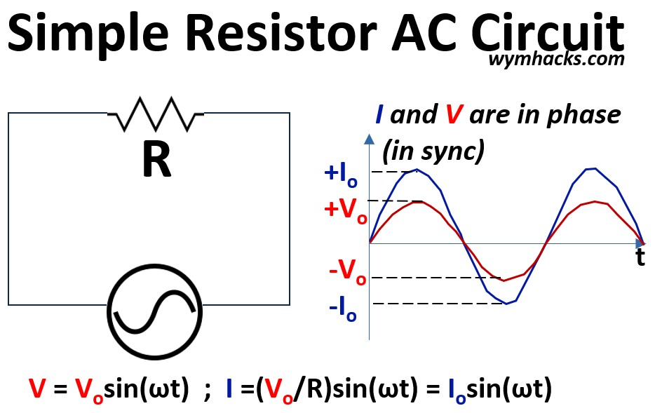
Note: Since I and V have different units of measure don’t try to compare the magnitude of the curves (apples and oranges).
- We put them together on the same chart to show that over time they move together in sync.
- We cant say anything about their relative magnitudes because they have different units.
Voltage and Current Equations
(1) V = V0sin(ωt) ; Voltage Equation Pure Resistive AC Circuit
- Since the largest value for sin (wt) will be one, V0 is the maximum voltage (the amplitude of the sinusoid)
Substituting V = IR (Ohm’s Law) into equation (1) gives
(2) I =(V0/R)sin(ωt) = I0sin(ωt) ; Current Equation Pure Resistive AC Circuit
See my post: AC Voltage and Current Equations for how these equations are derived.
Current and Voltage (i-v or I-V) Relationship
The voltage (V) and current (I) are perfectly in phase.
- This means they rise, fall, and cross zero at the exact same moment.
- i.e. the current is oscillating in sync with the voltage (and vice versa of course)
Opposition to AC
The circuit’s opposition to AC in a purely resistance circuit is equal to its resistance (R).
- We could call this resistance impedance as well (Z) but it’s not very useful to do so.
- Impedance is the total opposition to AC, encompassing the overall effect of all elements in a circuit.
- So we’ll come back to it later when we deal with more complicated circuit element configurations. (like R.L.C circuits)
Power
All electrical energy supplied to the resistor is dissipated as heat (real power).
The average power, P, is the actual power that is dissipated by the resistor as heat.
(3a) P = (Vrms)(Irms)
(3b) P = (Irms)2 R
(3c) P= (Vrms)2/R
Where:
- P is the Average Power (or Real Power) in Watts (W).
- Vrms is the Root Mean Square voltage in Volts (V).
- See my blog RMS (Root Mean Square) of a Sinusoid for more on RMS
- Irms is the Root Mean Square current in Amperes (A).
- R is the Resistance in Ohms Omega).
Pure Inductor AC Circuit – Time Domain Analysis
I primarily used these excellent Khan Academy Videos to write this section:
A purely inductive AC circuit contains only an inductor (L), which is an ideal coil with no resistance.
An inductor opposes changes in the current flowing through it.
In an AC circuit, the current is constantly changing, so the inductor generates a back electromotive force (EMF) that opposes the source voltage.
This opposition to AC current flow is called inductive reactance (XL).
This causes the I and V sinusoids to become out of sync.
An inductor does not consume any real power; it simply stores energy in its magnetic field and then releases it.
Picture: Simple (Pure) Inductor AC Circuit
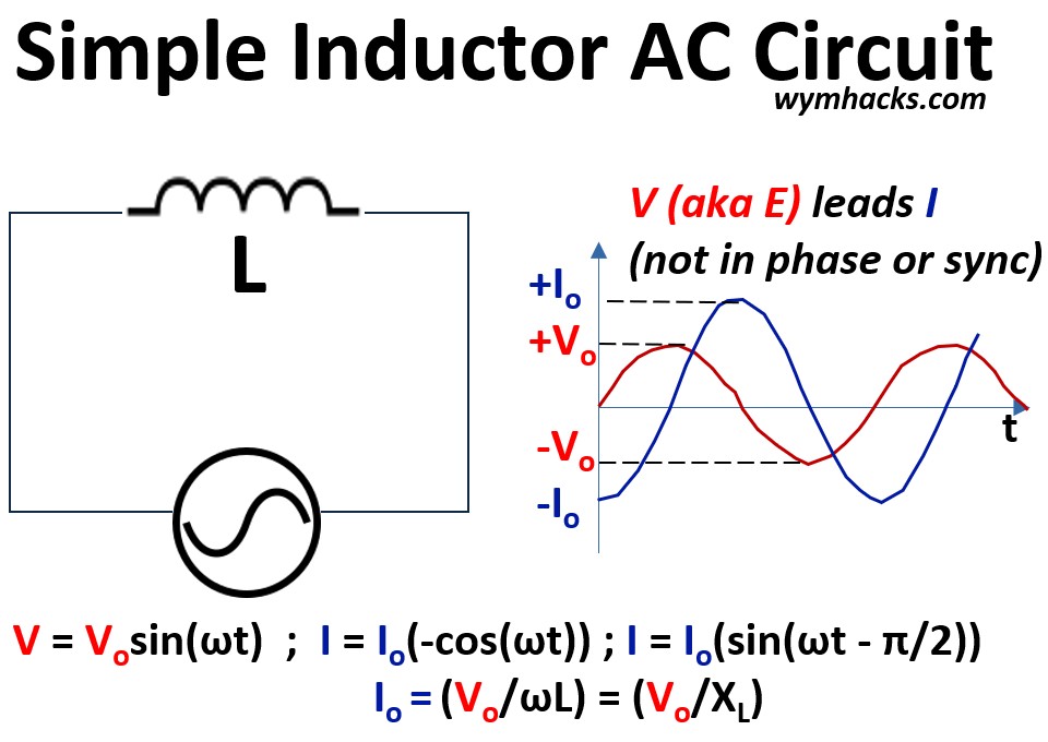
Note: Since I and V have different units of measure don’t try to compare the magnitude of the curves (apples and oranges).
- We put them together on the same chart to show that over time they do not move together in sync.
Voltage and Current Equations
The equation below is a mathematical expression of Faraday’s Law of Induction and Lenz’s Law as applied to a coil (inductor).
(4) VL= L dI/dt ; Inductor Voltage
It describes the instantaneous voltage VL across the inductor in terms of the rate of change of the current I passing through it
- VL = the instantaneous voltage across the inductor (in Volts)
- L = the inductance (a constant property of the coil) in units of Henrys (H).
- dI/dt = the instantaneous rate of change of current with respect to time in Amperes per second (A/s)
In a pure inductor circuit, the source voltage VS is equal to the voltage across the inductor VL.
(5) VL = VS
(6) VL = VS = V = Vosin(ωt) ; Voltage Equation for Pure Inductive AC Circuit
Combing (4) and (6) we get
(7) L dI/dt = V0sin(ωt)
Since integration is the inverse operation of differentiation, integrating both sides of the differential equation (7) is the standard procedure used to recover the original function whose derivative is given.
∫dI = ∫(V0/L)sin(ωt)dt
The solution to this integration is given below (see Example 1 in my blog Integration Definition and Rules for the detailed solution).
I = (V0/L)(-cos(ωt)/ω) + C
If we let V0 = 0, then I = C, but current is zero so I is zero, so C = 0.
- With C = 0 and rearranging the ω, we get
(8) I = (V0/(Lω))(-cos(ωt))
Let
(8b) I0 = (V0/(ωL))
so (8) becomes
(9) I =I0(-cost(ωt)); Current Equation Pure Inductive AC Circuit
Let’s express (9) in terms of the sine function so we can easily compare it to the voltage equation.
From our list of useful cosine and sine equivalences (Geometry and Trigonometry Rules) ,
-cos(θ) = sin(θ – π/2) , so substituting into (9) gives
(10) I = I0 sin(ωt– π/2) ; Current Equation Pure Inductive AC Circuit
So, let’s compare equations (6) and (10) and see if they explain the I and V graphs in the picture above.
(6) V = VS = VL = V0sin(ωt)
Equation (10) compared to (6) says that the current I oscillates 90 degrees (π/2 radians) behind the voltage.
That is, I is lagging behind Voltage (I lags V).
- If you take a look at the picture above, the way to find the leading curve is to start at time zero and see which value gets to zero or maximum first.
- In this case, V is ahead of I so V lead I or I lags V.
- Think of it this way: The inertia of the inductor is preventing I from instantly going up when V goes up.
Inductive Reactance XL
The term Lω in equation 8 is called the Inductive Reactance and is given the symbol XL.
Inductive Reactance XL is the opposition an inductor presents to the flow of Alternating Current (AC).
The value of XL is directly proportional to both the frequency of the AC signal and the inductance of the coil
(11) ωL = (2πf)L = XL = Inductive Reactance
- ω = angular velocity = 2πf
- f is the frequency (Hertz),
- L is the inductance (Henrys).
This relationship means an inductor offers zero opposition to DC (where f = 0) and higher opposition to high-frequency AC
- XL depends on the frequency of voltage source
- R does not depend on the frequency of voltage source
XL is measured in Ohms similar to resistance, but unlike resistance, it does not dissipate energy as heat;
- instead, it causes the current to lag the voltage by 90 degrees and
- stores energy in a magnetic field.
Since (see equation 8b)
(12a) I0 = (V0/(ωL)) ; Pure Inductor AC Circuit Version of Ohm’s Law
we can express this as
(12b) I0 = (V0/XL) ; Pure Inductor AC Circuit Version of Ohm’s Law
This equation is the AC (Alternating Current) version of Ohm’s Law for a circuit that contains only a pure inductor.
Power
Real Power (or True Power) is the power dissipated as heat or converted to useful work.
(13) Preal = VrmsIrmscos(θ)
- P is the Average Power (or Real Power) in Watts (W).
- Vrms is the Root Mean Square voltage in Volts (V).
- See my blog RMS (Root Mean Square) of a Sinusoid for more on RMS
- Irms is the Root Mean Square current in Amperes (A).
For a pure inductor, the phase angle θ (between V and I) is 90 degrees.
(13b) Preal = V I cos(90) = 0 Watts ; Pure Inductive AC Circuit Real Power
The zero real power means the inductor, like the capacitor, does not consume energy permanently.
Instead, it engages in an oscillating energy exchange with the AC source:
- Absorption: During one-quarter of the AC cycle, the source supplies energy to the inductor, which is stored in its magnetic field.
- Return: During the next quarter-cycle, the magnetic field collapses, and the inductor releases an equal amount of energy back to the AC source.
Because the energy is only stored and returned—and not converted to heat or work—the net amount of energy consumed over a full AC cycle is zero, resulting in zero real power
So, the average power consumed by a theoretically pure inductor over a full cycle is zero.
Pure Capacitor AC Circuit – Time Domain Analysis
I primarily used these excellent Khan Academy Videos to write this section:
A pure capacitor AC circuit is an idealized electrical circuit where an alternating current (AC) voltage source is connected to a circuit containing only a capacitor and no other opposition to current flow, such as resistance or inductance.
A capacitor opposes changes in voltage.
In an AC circuit, the voltage is constantly changing, so a current flows as the capacitor continually charges and discharges.
This opposition to AC current flow is called capacitive reactance XC.
This causes the I and V sinusoids to become out of sync.
In a purely capacitive circuit, the capacitor does not consume any real power; it simply stores and releases electrical energy.
Picture: Pure (Simple) Capacitor AC Circuit
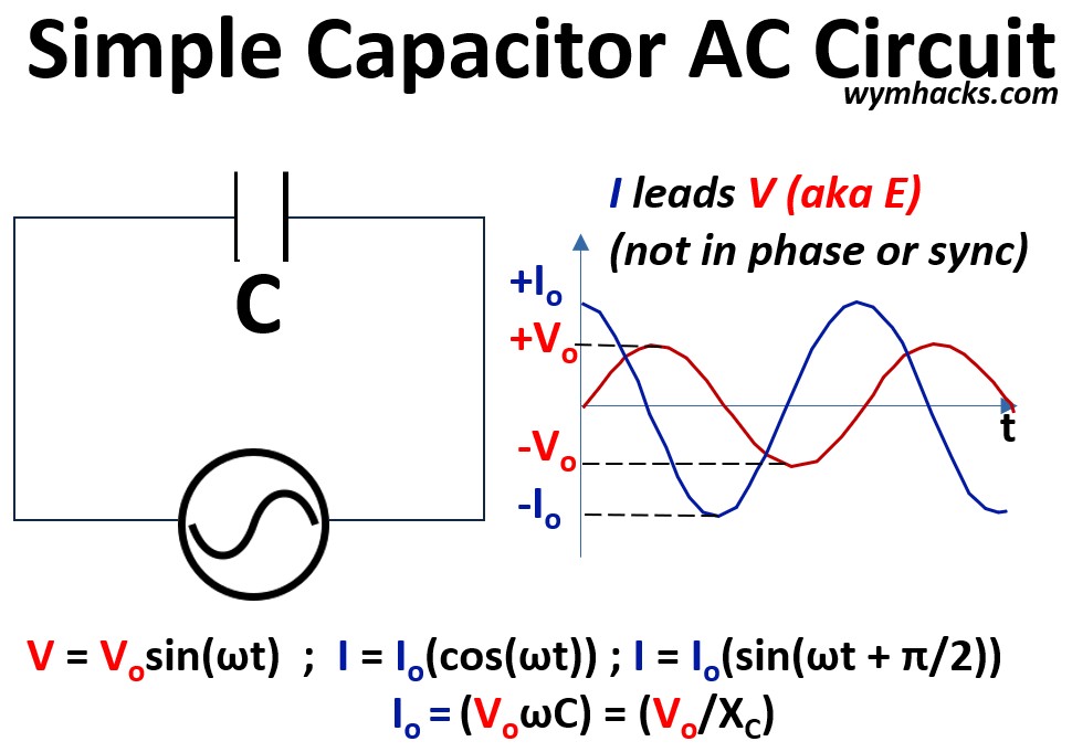
Note: Since I and V have different units of measure don’t try to compare the magnitude of the curves (apples and oranges).
- We put them together on the same chart to show that over time they do not move together in sync.
Voltage and Current Equations
In a purely inductive circuit the source voltage VS and capacitor voltage VC are equal
(14) VC = VS
(15) VS = V0sin(ωt) ; Voltage Equation for Pure Capacitive AC Circuit
Voltage in a capacitor is defined as follows (see my blog Capacitance for more)
(16) VC = Q/C ; Capacitor Voltage
Where
- Q = represents the electric charge stored on one plate of the capacitor (measured in Coulombs, C).
- C = Capacitance and has units of Farad.
Substituting (15) and (16) into (14) and solving for Q gives
(17) Q = CV0sin(ωt)
For an AC system (i.e. a continuously oscillating system) the definition of current will be
(18) I = dQ/dt ; AC Current
Substitute (17) into (18)
(19) I = d/dt(CV0sin(ωt))
- See Example 4 (chain rule example) in my blog The Derivative to see how to differentiate this.
- The differential of the right hand side of equation (19) with respect to t is
(20) I = ωCV0cos(ωt) ; Current Equation for a Pure Capacitive AC Circuit
Sine the max value for cosine is 1, that means that I max or I peak, I0 , is limited to ωCV0
(21) I0 = ωCV0
So (20) can be expressed as
(22) I = I0cos(ωt) ; Current Equation for a Pure Capacitive AC Circuit
We want to compare equation (22) with the voltage equation (15) so lets express the cosine function in (22) in terms of sine.
From my blog Geometry and Trigonometry Rules we know that cos(ωt) = sin(ωt + π/2), so (22) can be expressed as
(23) I = I0sin(ωt + π/2) ; Current Equation for a Pure Capacitive AC Circuit
(15) VS = VC = V0sin(ωt)
We see that for a capacitor circuit (see the picture graph above), the current I is oscillating ahead of the voltage.
This is the defining characteristic of a purely capacitive component and is opposite to the behavior of an inductor (where voltage leads current).
- I leads V
- V lags I
- From time = zero, I reaches zero and max before V does
- Think of it this way:
- A change in the voltage of the capacitor means the charge must change.
- To change the charge, a current must first occur, so its going to lead voltage.
Capacitive Reactance XC
Capacitive Reactance (XC) is the opposition a capacitor presents to the flow of Alternating Current (AC).
Unlike a resistor, which dissipates energy as heat, a capacitor’s opposition comes from its ability to store and release energy in an electric field.
This process is continuous in an AC circuit as the capacitor constantly charges and discharges, effectively limiting the AC current.
It is measured in Ohms, just like resistance, but is referred to as “reactance” to indicate it’s an opposition that is dependent on the signal frequency.
Capacitive reactance is calculated using the formula:
(24) XC = 1/(ωC) = 1/(2πfC) ; Capacitive Reactance
where
- XC = Capacitive Reactance in Ohms (Ω)
- ω = angular velocity in radians/s
- f = frequency of AC signal in Hertz (Hz)
- C = Capacitance in Farads (F)
The formula shows that XC is inversely proportional to frequency:
- f ↑ , XC ↓
- f ↓ , XC ↑
At high frequencies, the capacitor has little time to fully charge before the voltage polarity reverses, so it acts almost like a short circuit (low opposition).
At low frequencies the capacitor fully charges and acts like an open circuit (infinite opposition), effectively blocking DC and low-frequency signals.
Let’s come back to our peak current definition (see equation 21).
(21) I0 = ωCV0 ; Pure Capacitor AC Circuit Version of Ohm’s Law
This equation is the AC (Alternating Current) version of Ohm’s Law for a circuit that contains only a pure capacitor.
Where
- I0 = the peak current (the maximum current value in the cycle (Amperes)
- V0 = the peak voltage (the maximum voltage value in the cycle), measured in Volts
- ω is the angular velocity of the AC source, measured in radians per second
- C is the capacitance of the capacitor, measured in Farads (F).
we can express this using the Capacitive Reactance definition.
(25) I0 = (V0/XC) ; Pure Capacitor AC Circuit Version of Ohm’s Law
Power
Capacitive reactance does not consume real power.
In a purely capacitive circuit, the current I leads the voltage V by a phase angle of 90 degrees (π/2 radians).
Real Power (or True Power) is the power dissipated as heat or converted to useful work.
(26a) Preal = Vrms Irms cos(θ)
In a pure capacitor circuit, θ = – 90 degrees so
(26b) Preal = 0 ; Pure Capacitive AC Circuit
- P is the Average Power (or Real Power) in Watts (W).
- Vrms is the Root Mean Square voltage in Volts (V).
- See my blog RMS (Root Mean Square) of a Sinusoid for more on RMS
- Irms is the Root Mean Square current in Amperes (A).
The capacitor
- absorbs energy from the source during one-quarter of the AC cycle (when it’s charging) and
- immediately returns an equal amount of energy to the source during the next quarter-cycle (when it’s discharging).
Because the energy is only stored and returned, and not consumed or dissipated as heat (like in a resistor), the net power consumed over a full cycle is zero.
Phasor Basics
See this great introductory video
AC Circuits get interesting (and practical) when we start combining resistors, inductors, and capacitors.
We call these RLC AC circuits and I want to describe some basic relationships between current and voltage in these kinds of systems.
In order to do this we will need to use a tool called the Phasor and apply some basic vector math.
Phasor Characteristics
Consider a vector (something that has direction and magnitude….see my blog on vectors) which has the following characteristics:
- It’s rotating in a counterclockwise direction tracing a circular path.
- The tail of the vector is fixed at the center of the circle.
- The tip of the vector starts on the positive x axis
- in what we typically call quadrant I of the circle.
- The vector’s magnitude is equal to the amplitude (peak value) of a sinusoid wave equation like the ones representing voltage and current
- If V = V0sin(ωt), then vector magnitude = V0
- I = I0sin(ωt), then vector magnitude = I0
Over time, as the vector rotates in the counterclockwise direction it will project a pattern of instantaneous points in time which we can graph.
Picture: A Phasor Projects A Sinusoid Over Time
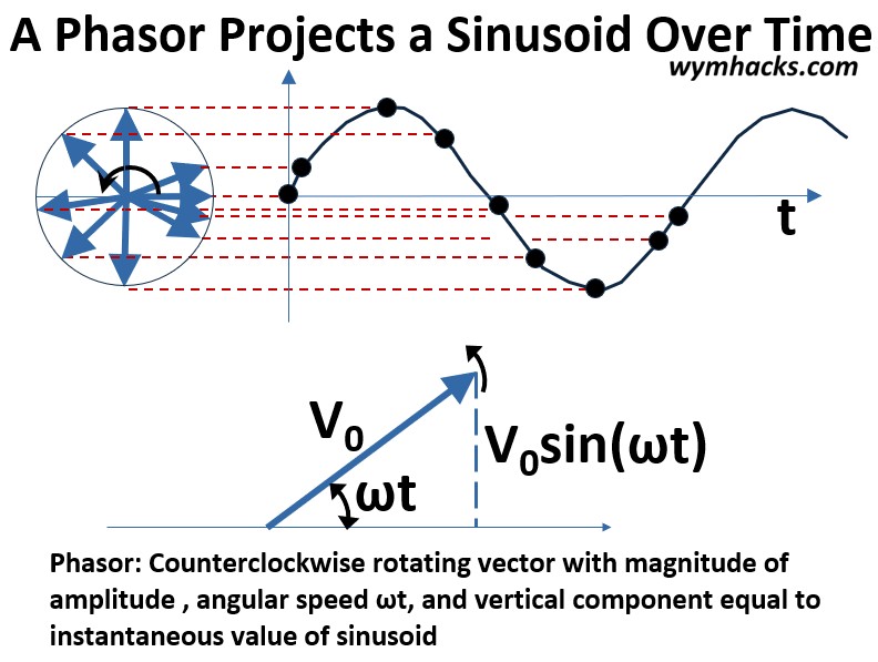
As the vector rotates , we can plot its y (vertical component) value on a graph of value (voltage or current) vs time.
- The projection of the value from the vector to the graph is shown by the red dotted lines.
- Cool. We get a sine or cosine shape over time which is exactly how we characterize current and voltage in AC circuits.
Assume the vector represents the voltage.
Freeze the vector at a specific position in time as shown in the picture above.
- We can characterize it as a right angle triangle with
- ωt: The angle between the vector and the 0 line is equal to the angular velocity x time (rad/sec x sec = radians).
- y component of vector: V0sin(ωt)
- We just applied the Pythagorean theorem to get this. (sin x = opposite/hypotenuse)
- See my trig blog if you need to remember what that is.
This rotating vector analogy is called a phasor.
Vector Math
We’ll have to add phasors in our study of RLC circuits but this is just vector addition and its pretty straight forward.
To add two vectors (let’s say A + B), you simply
- move “A” such that the tail of “A” connects to the tip of “B” and
- trace a new vector from the tail of “B” to the tip of the moved vector “A”.
- The new vector is “A + B”
Go to my blog Vector Math to get clear on this if you’re still confused.
Voltage and Current Relationships in RLC Circuits
While phasors are actually powerful tools rooted in complex number mathematics (which allows engineers to solve intricate AC circuits using simple algebra instead of calculus), we can simplify the concept for visual analysis.
We don’t need complex math to show how current and voltage either lag or lead each other in RLC circuits.
We can simply use the phasor vectors to represent the peak values and phase angles of currents and voltages and then use simple vector addition to derive the fundamental phase relationships for series and parallel RLC circuit basics.
These simple vector diagrams allow us to instantly see the overall phase relationship between total voltage and total current.
Series RLC AC Circuits (Voltage → Impedance → Power Triangles)
Here are some nice references re RLC Circuits.
- Impedance & phase angle of series L.C.R circuit – Khanacademy
- RLC Circuit: Series and Parallel, Applied circuits
We’ve reviewed pure, singular, resistive, inductive, and capacitive AC circuits and established phase relationships and learned about resistance (R) and reactance (XC and XL ).
Let’s combine these elements in AC circuits and learn a few more things.
A series RLC circuit is one of the most fundamental and crucial circuits in electrical engineering.
It gets its name from its three main components, all connected end-to-end (in series) to an AC voltage source:
- R for Resistor
- L for Inductor
- C for Capacitor
Picture: Series RLC AC Circuit
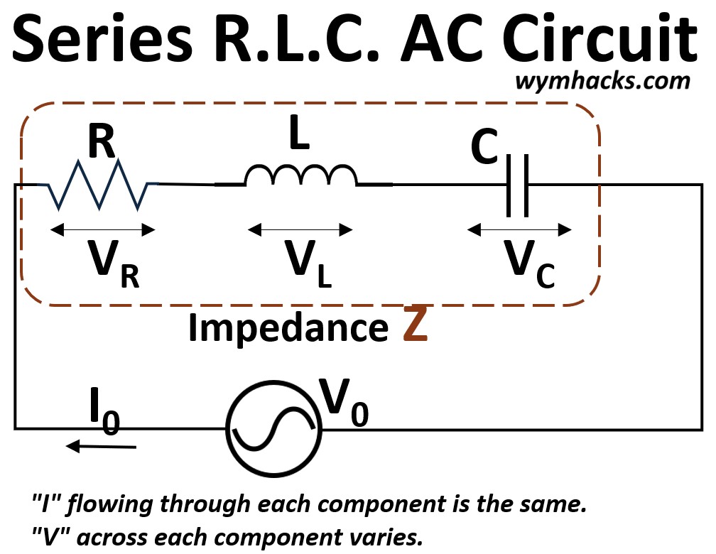
Series RLC AC Circuit Characteristics
Common Current
Since the components are in series, the same alternating current (I) flows through every single component at any given instant.
Voltages
By Kirchhoff’s Voltage Law (KVL), the total source voltage VS is the vector sum of the voltages across the resistor VR, the inductor VL, and the capacitor VC.
VS = VR + VL + VC is the vector sum of the voltages across the resistor (VR), the inductor (VL), and the capacitor (VC).
Because of the different phase relationships, this sum is not a simple arithmetic addition (i.e. have to use vector addition).
As we noted, the common current is usually the reference point for phase analysis.
You’ll notice the term Impedance in the picture above.
The impedance is a sort of composite resistance of the combined elements in the circuit.
We’ll address impedance later on, once we do a little vector math.
Series RLC Peak Voltage Calculation
Ok, remember those phasors we mentioned earlier on?
Well, we are going to use them to represent the position and magnitude of current and voltage in a series RLC circuit.
We noted that the current going through the components in a series R.L.C configuration will be the same.
Let’s create a reference phasor (vector) that represents this current I0 and we’ll place it flat on the x axis of a cartesian xy plane as shown in the picture below (see 1. in the picture).
Picture: Series AC RLC Peak Voltage Calculation
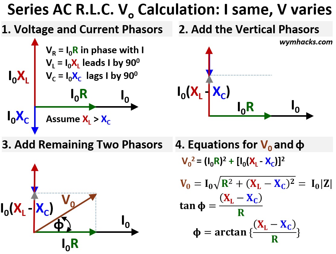
We can also define component voltage phasors and define them in terms of Ohm’s Law (in terms of resistance R or reactance X).
Resistor Voltage: VR = I0R
- This is the standard form of Ohm’s Law.
- The peak voltage VR across the resistor is directly proportional to the peak current I0 flowing through it and the resistance R.
- VR is in phase with the current I0
Inductor Voltage: VL = I0XL
- This is the Ohm’s Law equivalent for an inductor.
- The peak voltage VL across the inductor is proportional to the peak current I0 and the Inductive Reactance XL.
- VL leads the current I0 by 90 degrees (π/2 radians): Remember the mnemonic ELI the ICE man where E leads I in an inductor (L)
Capacitor Voltage: VC = I0XC
This is the Ohm’s Law equivalent for a capacitor.
- The peak voltage VC across the capacitor is proportional to the peak current I0 and the Capacitive Reactance XC.
- VC lags the current I0 by 90 degrees (π/2 radians): Remember the mnemonic ELI the ICE man where I leads E in a capacitor (C)
Now, lets place the phasors on the same xy plane and in relation to the current phasor I0.
You can see the voltage phasor (vector) placements as shown in 1. in the picture above where
- VR is in line with I0
- VL is +90 degrees ahead of I0
- Assume XL >XC (so VL >VC) although we could have chosen the opposite.
- VC is 90 degrees behind I0 (i.e. -90 degrees)
Add the Voltage Vectors Up
In order to compute the total voltage we have to add these vectors together.
Lets do VC + VL First.
- I show this in 2. in the picture above.
- Adding these two results in the vector I0(XL –XC)
- Move VC by the tail to the tip of VL
- then draw the resultant vector from the tail of VL to the tip of the moved VC.
- The resultant vector is also vertical but has a tip designated by the grey arrow in the picture.
- We’ re doing basic vector addition here (see my blog Vector Math).
- You can look at (XL –XC) as a net reactance term. You might sometimes see this expressed as Xnet .
Now let’s add the resultant vector I0(XL –XC) to the the remaining vector VR
- See 3. in the picture above.
- We do simple vector addition again (see my blog on vectors to understand how to add vectors)
- and get the resultant vector V0
Compute the Magnitude of V0 Using the Pythagorean Theorem
(V0)2 = (I0R)2 +(I0(XL –XC))2 ; Series AC R.L.C Circuit
V0 = I0 sqrt { (R)2 +(XL –XC)2 } ; Series AC R.L.C Circuit
|Z| = Magnitude of the Impedance = sqrt { (R)2 +(XL –XC)2 } so
V0 = I0|Z| ; Ohm’s Law Equivalent For Series AC RLC Circuit
- It states that the total peak voltage V0 is equal to the peak current I0 multiplied by the total magnitude of the Impedance |Z|.
- This equation ties together the voltage, current, and total opposition (impedance Z) for the entire AC circuit, just as V=IR does for a simple DC circuit.
Opposition
- Impedance (Z) measures how much a circuit impedes (opposes) the flow of electric current.
- Like resistance, impedance is measured in Ohms
- Components: Impedance combines two different types of opposition:
- Resistance (R): The opposition due to resistors, which converts energy into heat.
- Reactance (X): The opposition due to inductors XL and capacitors XC, which stores and releases energy (magnetic or electric).
- Direction (Phase): Unlike simple resistance, impedance is a vector (expressed algebraically as a complex number) because it includes a phase angle.
- This angle tells you whether the total voltage leads or lags the total current in the circuit.
Series RLC AC Circuit: V0 and I0 Phase Angle Φ
Lets solve for the phase angle Φ (see section 3 in the picture above).
- tan Φ = (XL – XC)/R
- Φ = arctan { (XL – XC)/R }
In the phasor setup we assumed that XL was larger than XC.
This means V will lead I in this series RLC circuit.
Using this equation, when XC > XL, Φ will be negative; indicating V lags I.
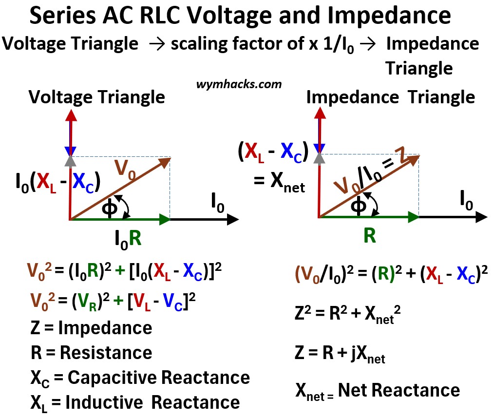
Series AC RLC Circuit: Voltage Triangle Scaled to the Impedance Triangle
I want to circle back to impedance again, to provide further clarity.
By applying the principles of vector addition to the voltages in a series RLC circuit, we established the relationship between the applied V0 and the individual component voltages VR ,VL ,VC.
This vector relationship forms a right triangle, which we can call the Voltage Triangle (as shown in 3. in the series RLC phasor picture above).
Since all these voltages share the same current, we can divide every side of this Voltage Triangle by I0 (using Ohm’s Law for AC circuits: V = IZ).
In a series RLC AC circuit, Ohm’s Law is expressed as: V = IZ where:
- V is the Source Voltage (usually given as an RMS or peak value).
- I is the Total Current flowing through the series loop.
- Z is the Impedance, representing the total opposition to current.
- In a DC circuit, resistance (R) is the only factor opposing current.
- However, in an AC circuit, two additional factors called reactances appear because of the changing nature of the current.
- Inductive Reactance (XL): The inductor opposes changes in current, causing the voltage to lead the current.
- Capacitive Reactance (XC): The capacitor opposes changes in voltage, causing the voltage to lag the current.
Since all these voltages share the same current, we can divide every side of this Voltage Triangle by I0 (using Ohm’s Law for AC circuits: V = IZ).
The result is a new, proportional right triangle (see the picture below) whose sides represent the circuit’s resistive and reactive properties:
- The side representing VR becomes the Resistance (R).
- The side representing the net reactive voltage (VL – VC) = I(XL – XC) becomes the Net Reactance (XL – XC = Xnet).
- The hypotenuse, which was V0, becomes the Impedance (Z): V/I = Z
This is the Impedance Triangle .
It demonstrates the Pythagorean relationship between these circuit elements: Z2 = R2+ Xnet2
The angle (Φ) between the Resistance (R) and the Impedance (Z) in this triangle is the phase angle of the circuit.
Picture: Series AC RLC Circuit Voltage Triangle Scaling to Impedance Triangle
Series AC RLC Circuit Impedance Z and the imaginary number j
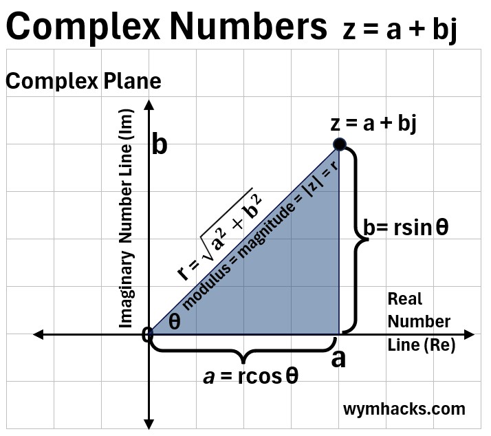
The Cartesian vector treatment we used—where the resistance vector (R) lies purely on the horizontal axis and the reactance vector (X) lies purely on the vertical axis—is a seamless precursor to the Complex Plane representation.
In the complex plane, the horizontal axis is called the real axis, and the vertical axis is called the imaginary axis.
This is where the mathematical operator j comes in:
- Resistance (R) is a real number and is placed on the real axis.
- Reactance (X) is always associated with a 900 phase shift (either leading for inductive, or lagging for capacitive).
- To represent this rotation mathematically, we multiply the reactance by j.
Thus, the imaginary number jXnet is placed on the imaginary axis.
This allows us to write the Impedance (Z) as a single complex number that incorporates both its magnitude (the hypotenuse) and its phase angle:
Z = R+ jXnet
The utility of j is that it mathematically incorporates the 900 phase angle that inherently exists between resistance and reactance, allowing us to perform all RLC circuit calculations using the standard algebra of complex numbers.
This transition confirms that the geometric vector addition we performed is mathematically equivalent to complex number addition.
- See my blogs on complex numbers: Complex Numbers; Complex Number Math; Circuit Analysis Math Basics
- Check out the picture below as a reminder of how to place a complex number in the complex plane
- Notice the equation for the magnitude of the hypotenuse (in the picture below).
- It will equate to the same |Z|= sqrt(R2+ Xnet2) we derived from the cartesian, phasor, vector analysis.
- Note that the magnitude of the complex number is the sqrt (the squares of the real and imaginary parts…not including j).
- The imaginary number operator j (j = sqrt(-1)) serves as the mathematical representation of that 900 phase separation.
Picture: Complex Numbers on the Complex Plane
Series AC RLC: Voltage Triangle Scaled to the Power Triangle
By applying the principles of vector addition to the voltages in a series RLC circuit, we established the relationship between the applied V0 and the individual component voltages VR ,VL ,VC.
As we observed in the previous section, this vector relationship forms a right triangle, which we can call the Voltage Triangle.
Knowing that voltage x current = power, we would like to convert or scale the voltage triangle into a power triangle.
Since the voltages share the same current, we can multiply every side of this Voltage Triangle by I0.
The result is a new, proportional right triangle (see the picture below) whose sides represent power expressions.
Picture: Series AC RLC Circuit Voltage Triangle to Power Triangle
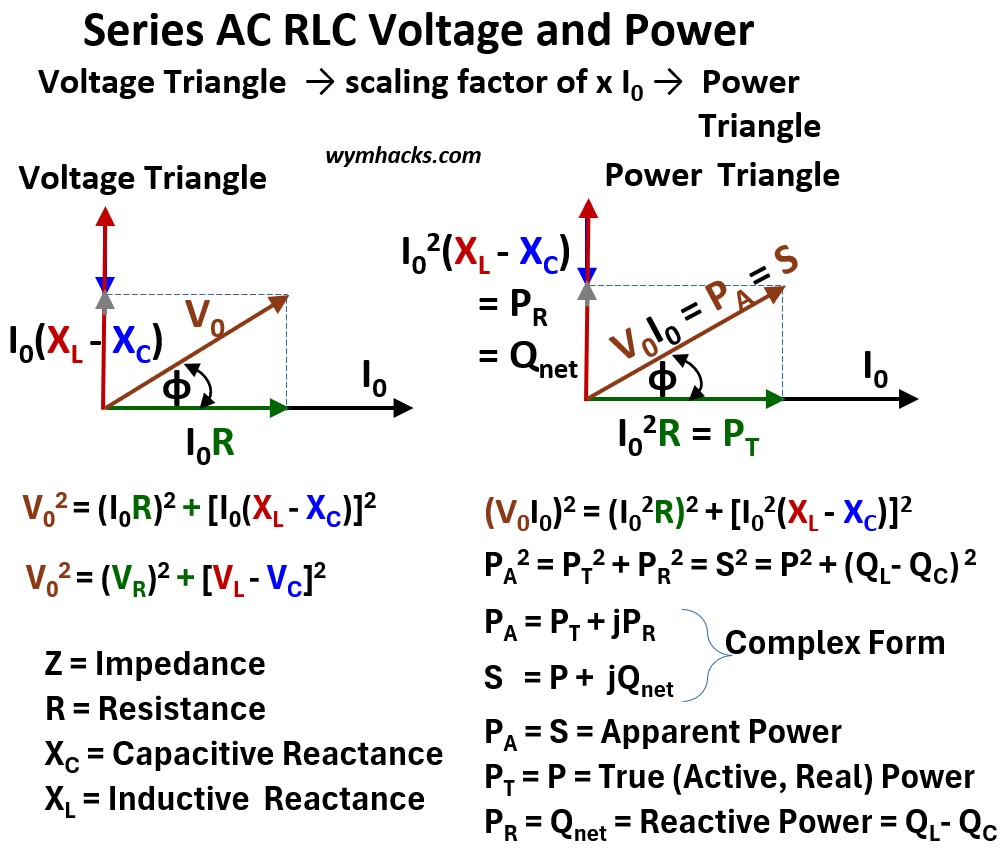
The side representing VR (= IR) becomes the True Power PT
- True Power is the useful power on the resistive part of the circuit.
- It is also called Active, Real, Actual, Useful, or Watt-full Power.
- The most common symbol for True Power is P.
The side representing the net reactive voltage (VL – VC) = I(XL – XC) becomes the Net Reactive Power = PR = I2(XL – XC) = QL – QC = Qnet.
- Net reactive power Qnet is the portion of electrical power that oscillates between the source and the load without being consumed.
- Qnet represents the net rate at which energy is temporarily stored and returned by the circuit’s inductive and capacitive fields.
- Also called Imaginary, Watt-less, Useless, or Quadrature Power (meaning 900 out of phase with True Power).
- The most common symbol for Reactive Power is Q (for quadrature I guess).
The hypotenuse, which was V0, becomes the Apparent Power PA
- Apparent power is the total magnitude of power delivered by the source,
- representing the vector sum of the Real Power dissipated by resistance
- and the Reactive Power oscillating within the system’s magnetic and electric fields.
- Also called Total Power, Complex Power Magnitude or Vector Power.
- The most commonly used symbol is S.
I used my own naming convention in this article for power so just remember that
- PT = P = True or Real or Actual or Useful Power
- PR = Q = Reactive or Imaginary or Watt-less or Useless or Quadrature Power
- PA = S = Apparent or Total or Complex Power Magnitude or Vector Power
This is the Power Triangle.
The Power Triangle is essentially a scaled version of the voltage triangle, where every side is multiplied by the circuit current I.
While the voltage triangle represents the distribution of potential drops, the power triangle represents the distribution of energy flow throughout the same components.
The angle Φ in a Series RLC AC Circuit
The general definition of the power factor (PF) that applies to every AC circuit—regardless of whether it is series, parallel, or a complex combination—is the ratio of Real Power (P) to Apparent Power (S).
- Power Factor (PF) = P/S = cos(Φ)
The power factor always describes two things:
Efficiency: It represents the percentage of the total power supplied (Apparent Power, in Volt-Amps or VA) that is actually converted into useful work or heat (Real Power, in Watts).
Phase Relationship: It represents the cosine of the phase angle ($\phi$) between the total supply voltage and the total supply current.
In a series RLC circuit, the angle Φ is a single value that represents the phase shift between the total supply current (which is common to all components) and the total supply voltage, and it can be visualized through three specific triangles:
- The Voltage Triangle
- Φ is the angle between the horizontal resistive voltage VR = IoR and the hypotenuse total supply voltage Vo, describing how much the total voltage leads or lags the common current.
- The Impedance Triangle
- Φ is the angle between the horizontal resistance (R) and the hypotenuse total impedance (Z), representing the overall opposition to current flow relative to the resistive part.
- The Power Triangle
- Φ is the angle between the horizontal true or real power (PT = P, in Watts) and the hypotenuse apparent power (PA= S, in Volt-Amps).
The circuit’s Power Factor PF =cos(Φ) can be computed from any of these triangles because they all have the same proportions:
- cos(Φ) = VR/VS
- cos(Φ) = R/Z = Resistance/Impedance
- cos(Φ) = P/S = PT /PA = True Power/Apparent Power
Series AC RLC Circuit: Summary
Ok, we covered a shit ton of ground…so let’s recap.
The picture below summarizes the series RLC AC circuit scaling process we described above.
Picture: Series RLC AC Circuit: Voltage, Impedance, and Power Triangles
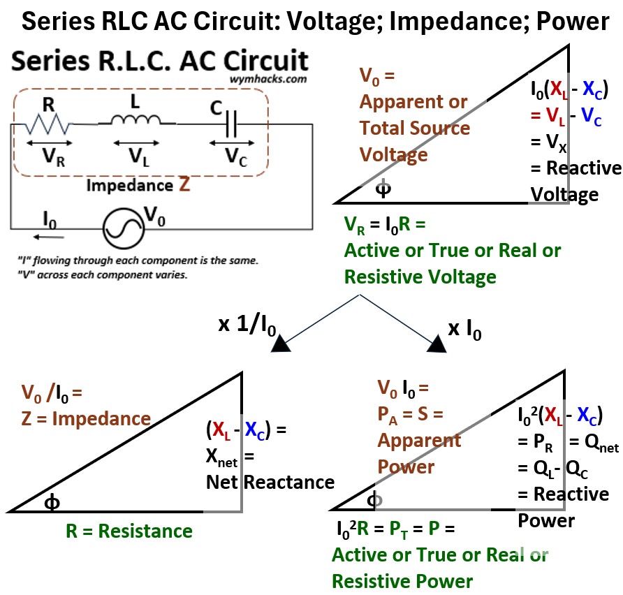
In AC circuit analysis, the relationship between these “triangles” is one of geometric scaling.
By applying Ohm’s Law and the Power Law to your initial measurements, you transform a triangle of “Flow” into a triangle of “Opposition” and finally into a triangle of “Energy.”
The Series RLC Path (Scaling the Voltage Triangle)
In a series circuit, we start with the Voltage Triangle, where
- VR is the horizontal,
- the net reactive voltage (VX = VL – VC) is the vertical, and
- V0 is the hypotenuse.
Voltage To Impedance: Since V = IZ, we divide every side of the Voltage Triangle by the constant current I.
This “shrinks” the triangle into the Impedance Triangle (with sides R, Xnet, Z), revealing the physical opposition of the components.
Voltage To Power: To find the energy usage, we multiply the original Voltage Triangle sides by the constant current I.
This “expands” the triangle into the Power Triangle, converting the voltages into Real Power P = PT, Reactive Power Qnet), and Apparent Power (S).
Power Factor RLC AC Circuit
In an RLC series circuit, the power factor cos(Φ) is
- the ratio of real power to apparent power,
- representing how effectively the circuit converts electrical energy into useful work.
- It is mathematically equivalent to the ratio of resistance to total impedance (R/Z).
- The power factor is categorized into three states based on the circuit’s dominant components:
- Lagging: If the inductor dominates (XL > XC), the current lags the voltage.
- Leading: If the capacitor dominates (XC > XL), the current leads the voltage.
- Unity: At resonance (XL = XC),
- the reactive components cancel out perfectly,
- the power factor becomes 1.0,
- and the circuit behaves as a purely resistive load where efficiency is maximized.
Parallel RLC AC Circuits (Current → Admittance → Power Triangles)
Here is a nice reference on RLC Circuits:
A parallel RLC circuit is another fundamental configuration in AC analysis.
It features the same three components—a resistor, an inductor, and a capacitor—but they are connected across the same two points, meaning they are arranged in parallel to the AC voltage source.
Picture: Parallel R.L.C. AC Circuit
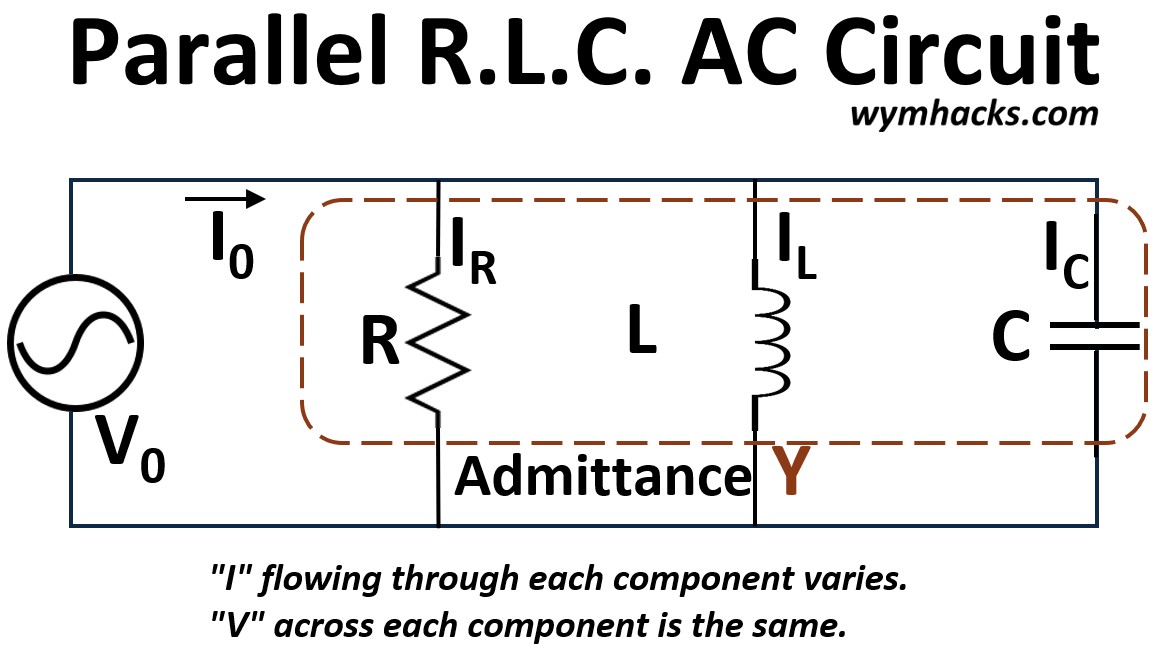
Parallel RLC AC Circuit Characteristics
Common Voltage
Since the components are in parallel, the same alternating voltage V is applied across every single component at any given instant.
This common voltage is typically the reference point for phase analysis.
Currents
By Kirchhoff’s Current Law (KCL), the total source current IS is the vector sum of the individual currents flowing through the resistor IR, the inductor IL, and the capacitor IC .
IS = IR + IL + IC
Because of the different phase relationships, this sum is not a simple arithmetic addition (must use vector addition).
As we noted, the common current is usually the reference point for phase analysis.
You’ll notice the term Admittance (Y) in the picture above.
While Impedance is opposition to current flow, Admittance is a measure of the ease of current flow.
We’ll address Admittance later on, once we do a little vector math.
Parallel AC R.L.C. Peak Current Calculation
The voltage across the components in a parallel R.L.C configuration will be the same.
Let’s create a reference phasor (vector) that represents this voltage and we’ll place it flat on the x axis of a cartesian xy plane as shown in the picture below (see section 1).
Picture: Parallel AC R.L.C. Peak Current Calculation
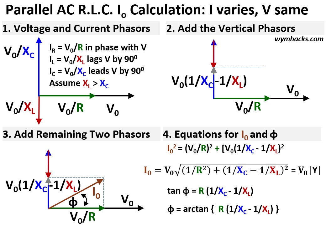
We can also define component current phasors and define them in terms of Ohm’s Law (in terms of resistance or reactance):
Resistor Current: IR = V0/R
- This is the standard Ohm’s Law for resistance.
- The peak current is determined solely by the common peak voltage V0 and the Resistance R.
- The current IR is in phase (0 degrees) with V0
Inductor Current : IL = V0/XL
- This is the Ohm’s Law equivalent for the inductor.
- The peak current is limited by the Inductive Reactance XL .
- The current IL lags the common voltage V0 by 90 degrees.
Capacitor Current : IC = V0/XC
- This is the Ohm’s Law equivalent for the capacitor.
- The peak current is limited by the Capacitive Reactance XC.
- The current IC leads the common voltage V by 90 degrees
Now, lets place the phasors on the same xy plane and in relation to the voltage phasor V0.
You can see the voltage phase (vector) placements as shown in section 1 of the picture above where
- IR is in line with V0
- IL is -90 degrees behind V0
- Like for the series RLC, Assume XL > XC so, IL < IC
- IC is 90 degrees ahead of V0 (i,e +90 degrees)
Add the Current Vectors (Phasors) Up
In order to compute the total voltage we have to add these vectors together.
Lets do IC + IL First.
- I show this in section 2 of the picture above.
- Adding these two results in the vector V0(1/XC -1/XL)
- (1/XC -1/XL) is called the net susceptance.
Now lets add the resultant vector V0(1/XC -1/XL) to the the remaining vector V0/R
- See section 3 in the picture above.
- We do simple vector addition again (see my blog on vectors to understand how to add vectors)
- and get the resultant vector I0
Compute the Magnitude of I0 Using the Pythagorean Theorem
(I0)2 = (V0/R)2 +(V0(1/XC -1/XL))2 ; Parallel AC RLC
I0 = V0 sqrt { (1/R)2 + (1/XC -1/XL)2 } ; Parallel AC RLC
Let |Y| = Magnitude of the Admittance = sqrt { (1/R)2 + (1/XC -1/XL)2 } so
I0 = V0|Y| ; Ohm’s Law Equivalent For Parallel AC RLC Circuit
Common Names of Some Terms
- G = 1/R = Conductance
- BC= 1/XC = Capacitive Susceptance
- BL= 1/XL = Inductive Susceptance
- XC = Capacitive Reactance
- XL = Inductive Reactance
Admittance
As noted above, the square root term
sqrt { (1/R)2 + (1/XC -1/XL)2 }
represents the magnitude of the total Admittance |Y| for the circuit.
This term combines the Conductance (1/R) and the Net Susceptance (1/XC -1/XL) through vector addition, defining the circuit’s total ease of current flow.
V0 and I0 Phase Angle Φ for Series AC RLC Circuit
Lets solve for the phase angle Φ from section 3 in the picture above.
- tan Φ = R (1/XC – 1/XL )
- Φ = arctan { R(1/XC –1/XL) }
In the phasor setup we assumed that XL was larger than XC.
This means I will lead V in this parallel AC RLC circuit (+ Φ).
Using this equation, when XC > XL, Φ will be negative; indicating I lags V.
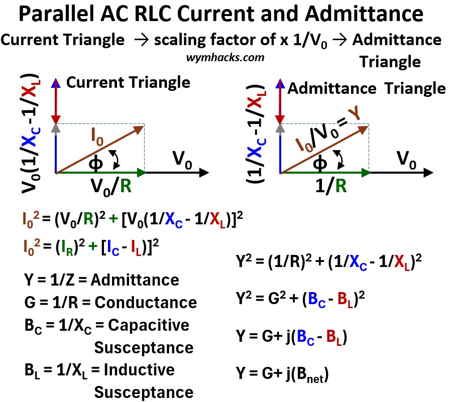
Current Triangle Scaled to the Admittance Triangle
Just as we did before for a series circuit, I want to circle back to the admittance again, to provide further clarity.
By applying the principles of vector addition to the currents in a parallel RLC circuit, we established the relationship between the applied I0 and the individual component currents IR ,IL ,IC.
This vector relationship forms a right triangle, which we can call the Current Triangle (as shown in 3. in the parallel RLC phasor picture above).
Since all these currents share the same voltage, we can divide every side of this Voltage Triangle by V0 (using Ohm’s Law for AC circuits: V = IZ).
The result is a new, proportional right triangle (see the picture below) whose sides represent the circuit’s resistive and reactive properties:
- The side representing IR becomes the 1/R = Conductance
- The side representing the net reactive current (IC – IL) becomes the Net Susceptance (1/XC – 1/XL = Bnet).
- The hypotenuse, which was I0, becomes the Admittance (Y): I/V = Y = 1/Z
This is the Admittance Triangle .
It demonstrates the Pythagorean relationship between these circuit elements: Y2 = (1/R)2+ Bnet2
The angle (Φ) between the Resistance (R) and the Admittance (Y) in this triangle is the phase angle of the circuit.
Picture: Parallel AC RLC Current and Admittance
Parallel AC RLC Admittance Y and the imaginary number j
The Cartesian vector treatment we used—where the conductance vector (G) lies purely on the horizontal axis and the susceptance vector (B) lies purely on the vertical axis—is a seamless precursor to the Complex Plane representation.
In the complex plane, the horizontal axis is called the real axis, and the vertical axis is called the imaginary axis.
This is where the mathematical operator j comes in:
- Conductance (G) is a real number and is placed on the real axis.
- Susceptance (B) is always associated with a 900 phase shift (either leading for inductive, or lagging for capacitive).
- To represent this rotation mathematically, we multiply the reactance by j.
Thus, the imaginary number jBnet is placed on the imaginary axis.
This allows us to write the Admittance (Y) as a single complex number that incorporates both its magnitude (the hypotenuse) and its phase angle:
Y= G+ jBnet
The utility of j is that it mathematically incorporates the 900 phase angle that inherently exists between conductance and susceptance, allowing us to perform all RLC circuit calculations using the standard algebra of complex numbers.
This transition confirms that the geometric vector addition we performed is mathematically equivalent to complex number addition.
- See my blogs on complex numbers: Complex Numbers; Complex Number Math; Circuit Analysis Math Basics
- Check out the picture below as a reminder of how to place a complex number in the complex plane
- Notice the equation for the magnitude of the hypotenuse (in the picture below).
- It will equate to the same |Y|= sqrt(G2+ Bnet2) we derived from the cartesian, phasor, vector analysis.
- Note that the magnitude of the complex number is the sqrt (the squares of the real and imaginary parts…not including j).
- The imaginary number operator j (j = sqrt(-1)) serves as the mathematical representation of that 900 phase separation.
Picture: Complex Numbers on the Complex Plane
Parallel AC RLC: Current Triangle Scaled to the Power Triangle
As we have seen above, by applying the principles of vector addition to the currents in a parallel RLC circuit, we established the relationship between the applied I0 and the individual component currents IR ,IL ,IC.
This vector relationship forms a right triangle, which we can call the Current Triangle
Knowing that voltage x current = power, we would like to convert or scale the current triangle into a power triangle.
Since all these currents share the same voltage, we can multiply every side of this Current Triangle by V0.
The result is a new, proportional right triangle (see the picture below) whose sides represent power expressions.
Picture: Parallel AC RLC Current Triangle to Power Triangle
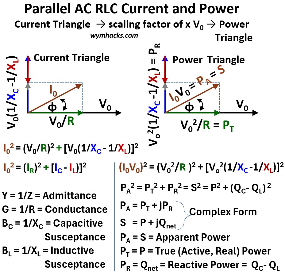
The side representing V0/R (= IR) becomes the True Power PT
- True Power is the useful power on the resistive part of the circuit.
- It is also called Active, Real, Actual, Useful, or Watt-full Power.
- The most common symbol for True Power is P.
The side representing the net reactive current (IC – IL) = V0(1/XC – 1/XL) becomes the Net Reactive Power = PR = V02(1/XC – 1/XL) = QC – QL = Qnet.
- Net reactive power Qnet is the portion of electrical power that oscillates between the source and the load without being consumed.
- Qnet represents the net rate at which energy is temporarily stored and returned by the circuit’s inductive and capacitive fields.
- Also called Imaginary, Watt-less, Useless, or Quadrature Power (meaning 900 out of phase with True Power).
- The most common symbol for Reactive Power is Q (for quadrature I guess).
The hypotenuse, which was I0, becomes the Apparent Power PA = I0V0
- Apparent power is the total magnitude of power delivered by the source,
- representing the vector sum of the Real Power dissipated by resistance
- and the Reactive Power oscillating within the system’s magnetic and electric fields.
- Also called Total Power, Complex Power Magnitude or Vector Power.
- The most commonly used symbol is S.
I used my own naming convention in this article for power so just remember that
- PT = P = True or Real or Actual or Useful Power
- PR = Q = Reactive or Imaginary or Watt-less or Useless or Quadrature Power
- PA = S = Apparent or Total or Complex Power Magnitude or Vector Power
This is the Power Triangle.
The Power Triangle is essentially a scaled version of the current triangle, where every side is multiplied by the circuit current V0.
While the current triangle represents the current flow, the power triangle represents the distribution of energy flow throughout the same components.
The angle Φ in a Parallel RLC circuit
The general definition of the power factor (PF) that applies to every AC circuit—regardless of whether it is series, parallel, or a complex combination—is the ratio of Real Power (P) to Apparent Power (S).
Power Factor (PF) = P/S = cos(Φ)
The power factor always describes two things:
- Efficiency: It represents the percentage of the total power supplied (Apparent Power, in Volt Amps or VA) that is actually converted into useful work or heat (Real Power, in Watts).
- Phase Relationship: It represents the cosine of the phase angle (Φ) between the total supply voltage and the total supply current.
In a parallel RLC circuit, the angle Φ is a single value that represents the phase shift between the total supply voltage (the same across each element) and the total supply current, and it can be visualized through three specific triangles:
- The Current Triangle
- Φ is the angle between the horizontal resistive current (IR) and the hypotenuse total supply current (I0), describing how much the total current leads or lags the common voltage.
- The Admittance Triangle
- Φ is the angle between the horizontal conductance (G = 1/R) and the hypotenuse total admittance (Y = I0/V0), representing the overall “ease” with which the circuit allows current to flow relative to its resistive parts.
- The Power Triangle
- Φ is the angle between the horizontal true or real power (P = PT, in Watts) and the hypotenuse apparent power (S = PA, in Volt Amps),
The circuit’s Power Factor PF = cos(Φ) can be computed from any of these triangles because they are all have the same proportions
- cos(Φ) = IR/I0 =
- cos(Φ) = G/Y = Conductance/Admittance
- cos(Φ) = PT/PA = P/S = True Power/Apparent Power
Parallel AC RLC: Summary
Picture: Parallel RLC AC Circuit: Current, Admittance, and Power Triangles
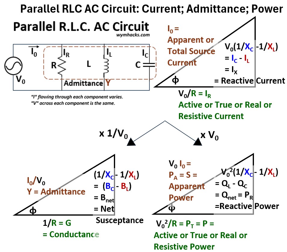
In AC circuit analysis, the relationship between these triangles is one of geometric scaling.
By applying Ohm’s Law and the Power Law to your initial measurements, you transform a triangle of “Flow” into a triangle of “Opposition” and finally into a triangle of “Energy.”
The Parallel RLC Path (Scaling the Current Triangle)
In a parallel circuit, the voltage V is the constant across all branches, so we start with the Current Triangle rather than a voltage triangle. In this geometry:
IR (Resistive Current) is the horizontal base.
The net reactive current (IXX = ICX – ILX) is the vertical leg.
Note that in parallel, capacitive current points upward and inductive current points downward, the inverse of the series configuration.
Itotal is the hypotenuse.
Current to Admittance: Since I = VY, we divide every side of the Current Triangle by the constant voltage V.
This transforms the triangle into the Admittance Triangle (with sides Conductance G, Susceptance B, and Admittance Y), revealing the total ease with which current flows through the parallel branches.
Current to Power: To find the energy usage, we multiply the sides of the Current Triangle by the constant voltage V.
This “expands” the triangle into the Power Triangle, converting the branch currents into Real Power (P), Reactive Power (Qnet), and Apparent Power (S).
Parallel RLC Power Factor
In a parallel RLC circuit, the power factor cos(Φ) remains the ratio of real power to apparent power, representing the system’s efficiency in performing useful work.
However, because the components are in parallel, the power factor is mathematically equivalent to the ratio of conductance to total admittance (G/Y).
The power factor is categorized into three states based on which branch draws the most current:
- Leading: If the capacitor dominates (XC < XL), the total current leads the voltage.
- Note that in parallel, the smaller impedance draws the larger current.
- Lagging: If the inductor dominates (XL < XC), the total current lags the voltage.
- Unity: At resonance (BL = BC or XL = XC), the inductive and capacitive currents cancel each other out perfectly.
- The power factor becomes 1.0, and the circuit behaves as a purely resistive load, drawing the minimum possible total current from the source.
The Universality of the Power Triangle
While these power equations are often introduced using simple series or parallel RLC circuits, they are actually fundamental laws of physics that apply to any single-phase AC system.
Picture: Power Triangle for any Single Phase AC Circuit
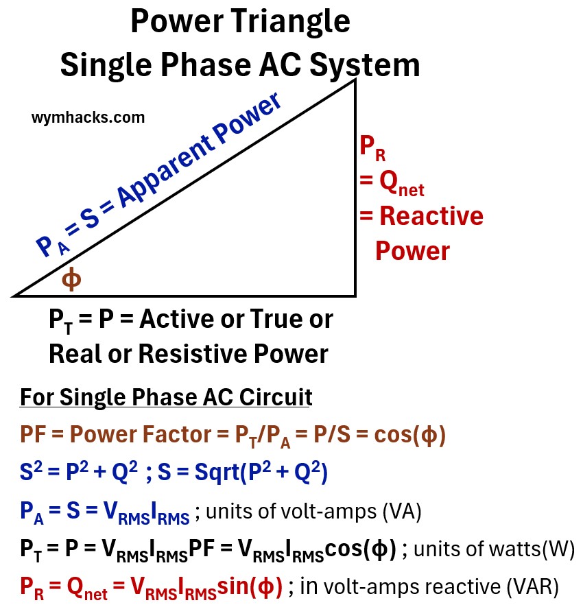
Whether a circuit contains three components or three hundred, these relationships remain constant for several key reasons:
1. The “Black Box” Principle
To an AC power source, a complex network of resistors, inductors, and capacitors behaves like a single, unified load.
This is often called “equivalent impedance.”
No matter how messy the wiring is inside the “box,” the source only “sees” two things: the total RMS Voltage it provides and the total RMS Current that results.
Because there is only one voltage and one current, there is only one phase angle (Φ) between them, which defines the Power Factor for the entire system.
2. Total Summation of Energy
The power triangle represents the total “energy budget” of a system:
- Real (True) Power (P): The total wattage is the simple sum of all energy converted to heat or work by every single resistor in the network.
- Reactive Power (Qnet or PR): This represents energy that is temporarily borrowed and then returned by magnetic and electric fields.
- Inductors and capacitors naturally “cancel” each other out.
- The Qnet is simply the final balance of that borrowed energy across the whole system.
3. Geometric Necessity
Because Real Power and Reactive Power act at a 90 degree offset—one performing work and the other maintaining fields—they will always form the legs of a right triangle.
- The Apparent Power (S) is the hypotenuse of that triangle.
- This isn’t just a rule for simple circuits; it is a mathematical requirement for how waves of voltage and current interact over time.
The Bottom Line:
- You do not need to know the internal layout of a circuit to use these formulas.
- If you can measure the voltage across the main terminals and the current entering the system, the Power Triangle will always accurately describe the relationship between the power used, the power stored, and the total power delivered.
Voltage, Current , Power Graphs: Derived From Series RLC Equation
Now let’s look at graphs of current, voltage, and power for a series RLC circuit.
I entered the following data points and equations into desmos.com:
Physics Sliders
- f=60
- R=10
- L=0.05
- C=0.0002
Visual Sliders
- Av=10 (Voltage Peak Height)
- Ai=7 (Current Peak Height)
- Ap=5 (Power Peak Height)
Calculated Logic
- ω=2πf
- XL=ωL
- XC=1/(ωC)
- ϕ=arctan((XL−XC)/R)
The Curves
- v(x)=Avsin(ωx)
- i(x)=Aisin(ωx−ϕ)
- p(x)= Apsin(ωx)sin(ωx−ϕ)
- yavg=0.5Apcos(ϕ) (Set this to a dashed line)
Given the inputs above, I generated the following slides showing the relationship between graphs of voltage, current, and power.
Picture: Purely Resistive State Derived From Series RLC Equation
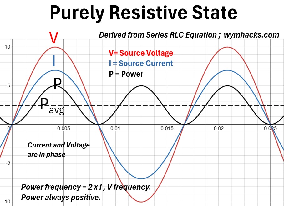
In a purely resistive RLC circuit (typically at resonance), the voltage and current curves are perfectly in-phase,
- meaning they reach their maximum, minimum, and zero points at the exact same time.
Because there is no phase shift (Φ = 0), the power factor (the fraction of total power that is doing actual work) is exactly 1 (ideally).
This synchronization ensures that the electrical energy is converted immediately and entirely into heat or work without any “sloshing” back and forth between the source and the components.
The power curve (P = VI) is the most distinct of the three:
- it oscillates at twice the frequency of the voltage or current but remains entirely positive.
- Since the voltage and current always have the same sign (both positive or both negative), their product is never negative.
- This means there is no negative power; energy only flows from the source to the resistor and is never returned.
The power curve sits entirely above the zero-axis, oscillating between zero and a peak value,
- resulting in a constant dissipation of “real power”
- where the average power is simply P = VRMSIRMS.
Picture: Purely Inductive State Derived From Series RLC Equation
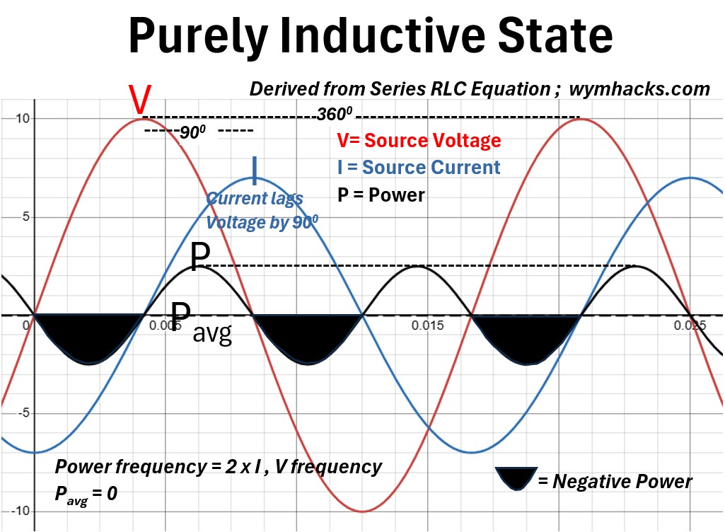
In a purely inductive state, the most critical characteristic is the 90° phase shift, where the voltage leads the current (or current lags voltage).
This means the current reaches its peak exactly one-quarter cycle after the voltage.
Consequently, the power curve—calculated as the instantaneous product of voltage and current (p = vi) oscillates at twice the system frequency and is centered perfectly at zero on the vertical axis.
Because the power curve spent equal time in the positive and negative regions, the average power (P) is zero.
- During the positive half-cycles of the power curve, the inductor is absorbing energy to build its magnetic field;
- during the negative half-cycles, it returns that exact same energy to the source as the field collapses.
- This signifies that no real work is being performed;
- the energy is simply “borrowed” and “returned,” which is why we describe the power in this state as purely reactive.
Picture: Purely Capacitive State Derived From Series RLC Equation
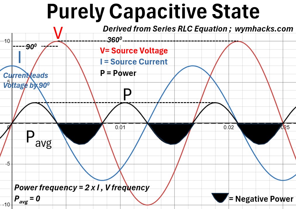
Waveform Shift
In a purely capacitive RLC state, the most critical characteristic is the 90 degree phase shift: the current waveform (I) leads the voltage waveform (V) by exactly one-quarter of a cycle.
This occurs because a capacitor opposes changes in voltage, requiring current to flow and build up charge before the voltage can rise.
Consequently, the current peaks when the voltage is at zero, and the voltage reaches its maximum only when the current has dropped back to zero.
Power Curve
The power curve (P), calculated as the instantaneous product of V and I, is a sine wave oscillating at twice the system frequency with an average value of zero.
Because the voltage and current are perfectly out of phase, the power alternates between positive and negative cycles of equal area;
- the capacitor absorbs energy from the source to create an electric field and then returns that exact amount of energy back to the source.
- This indicates that no Active Power (P) is consumed; instead, the circuit deals entirely in Reactive Power (Q), where energy simply surges back and forth without performing any real work.
Purely Capacitive vs Purely Inductive
When you compare a purely inductive circuit to a purely capacitive one (the last two graphs above), you see a total physical offset of their power curves.
- In an inductive circuit, the power curve is positive when the magnetic field is building;
- in a capacitive circuit, the power curve is negative at that exact same moment as the electric field collapses.
- This 180° opposition means that the two components are essentially playing a game of “catch” with energy.
- Because one is releasing energy while the other is absorbing it, the net reactive power (Qnet) the source has to provide is significantly reduced.
- This is the fundamental principle behind using capacitor banks in industrial plants:
- the capacitors provide the “sideways” reactive force (QC) that the motors’ inductors (QL) need,
- preventing that extra energy from having to travel all the way from the power plant
Picture: RL Circuit Derived From Series RLC Equation
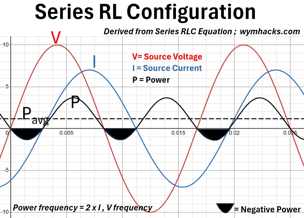
In an RL (inductive) state, the defining characteristic is that the current waveform (I) lags the voltage waveform (V) by a phase angle (Φ) between 0 and 90 degrees.
Unlike a purely inductive circuit, the presence of resistance prevents a full 90 degree shift.
The voltage reaches its peak first, followed by the current peak after a short delay.
This lag occurs because the inductor’s induced back-EMF opposes the initial flow of current, while the resistor dissipates energy simultaneously.
The power curve (P) reflects this “mixed” behavior by shifting vertically.
Unlike the purely reactive state where the power curve is centered at zero, the RL power curve has a positive average value, which represents the Active Power (P) being consumed by the resistor as heat.
While the curve still dips below the zero axis—indicating moments where the inductor returns stored magnetic energy to the source (Reactive Power (Qnet))
the area above the axis is significantly larger than the area below it.
This asymmetry confirms that the circuit is performing net work while also maintaining a pulsating magnetic field.
Picture: RC Circuit Derived From Series RLC Equation
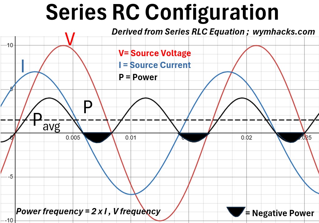
In an RC (Resistive-Capacitive) state, the key characteristic is that the current (I) leads the voltage (V) by a phase angle (Φ) somewhere between 0° and 90°.
Unlike a purely capacitive circuit, the presence of resistance prevents a perfect 90° shift; the current peaks before the voltage, but they partially overlap.
This overlap indicates that the circuit is no longer just storing and returning energy, but is now actively dissipating it.
The power curve (P) reflects this shift by oscillating at twice the system frequency, but with a crucial difference: it is now offset upward from the zero-axis.
While the curve still dips into the negative region (representing energy being returned by the capacitor), the positive portion of the cycle is much larger.
The area above the axis represents the Active Power (P) being permanently consumed by the resistor as heat, while the alternating portion represents the Reactive Power (Qnet) cycling through the capacitor.
The average value of this entire curve is no longer zero, but equals the real wattage of the circuit.
Picture: Inductive Dominant RLC Derived From Series RLC Equation
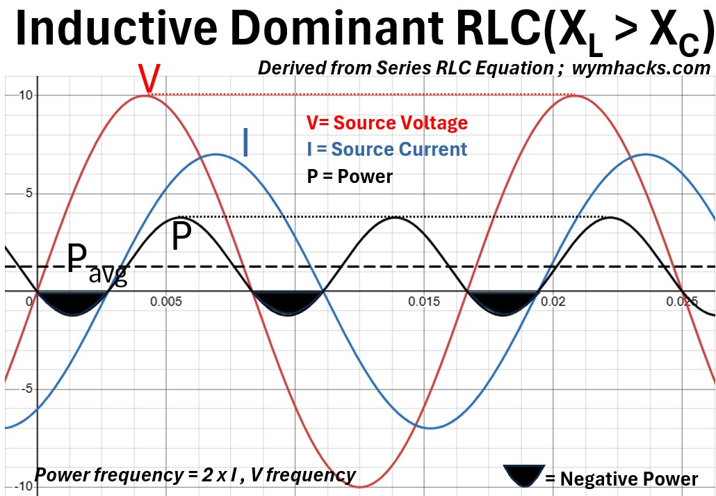
In an inductive-dominant RLC circuit, the defining characteristic is that the current waveform (I) lags the voltage waveform (V).
Because the inductor’s magnetic field opposes rapid changes in current, the current peak occurs shortly after the voltage peak.
The phase angle (Φ) is positive, and though it is less than the 90 degree shift seen in a purely inductive circuit due to the presence of resistance and capacitance, the “lagging” behavior remains the dominant trait.
The power curve (P) reflects this lag by shifting partially into the negative region, representing energy being returned to the source, but it remains predominantly positive.
Unlike a purely reactive circuit where the average power is zero, the presence of resistance ensures that the positive cycles of the power wave are larger than the negative cycles.
The vertical offset of this wave above the zero-axis represents the Active Power (P) being consumed by the resistor, while the oscillation between the source and the reactive components represents the Net Reactive Power (Qnet).
Picture: Capacitive Dominant RLC Derived From Series RLC Equation
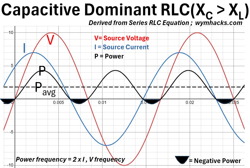
In a capacitive-dominant RLC circuit, the defining characteristic is that the current waveform (I) leads the voltage waveform (V).
Unlike a purely capacitive circuit where the lead is exactly 90 degrees, the presence of resistance and inductance pulls this phase angle (Φ) to a value between 0 and 90 degrees.
You will observe that the current peaks shortly before the voltage reaches its maximum, indicating that the capacitor’s charging effect is the dominant influence on the circuit’s timing.
The power curve (P) reveals the “Active” work being done.
Because the phase shift is less than 90 degrees, the power waveform is shifted upward, spending more time in the positive region than the negative.
The positive area represents energy consumed by the resistor as heat, while the negative area shows reactive energy being returned to the source by the capacitor and inductor.
The average value of this curve is no longer zero; it is a positive value equal to the Real Power (P), confirming that while energy is still oscillating (Reactive Power), actual work is being performed.
Picture: Balanced RLC (Resonance) Derived From Series RLC Equation
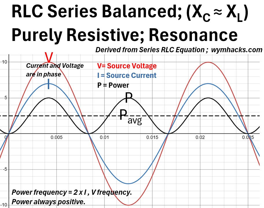
In a balanced RLC state, known as resonance, the inductive and capacitive reactances cancel each other out perfectly (XL = XC), making the circuit behave as a purely resistive load.
The key characteristic of the waveforms is that the voltage (V) and current (I) are exactly in phase; they reach their peak values and cross zero at the same moments.
Because there is no phase shift (Φ = 0)), the power factor is unity (cos(Φ ) = 1.0), and the circuit draws the minimum possible current for a given voltage.
The power curve (P) reflects this perfect alignment by remaining entirely positive (or zero), never dipping below the horizontal axis.
Unlike the purely reactive states where power oscillates back and forth, the power at resonance represents a continuous flow of energy into the resistor.
The instantaneous power peaks when both V and I peak, and its average value (Pavg) is exactly half of that peak.
In this state, the reactive power (Qnet) is zero because the energy being stored in the inductor’s magnetic field is provided entirely by the discharging capacitor, and vice versa, leaving the source to provide only the Active Power required by the resistance.
Summary Tables
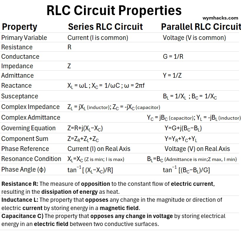
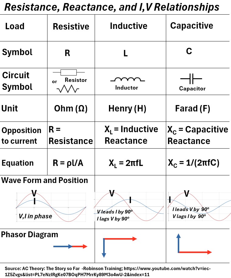
Picture: Resistance, Reactance and I,V Relationships Table
Picture: RLC Circuit Properties Table