Set Up
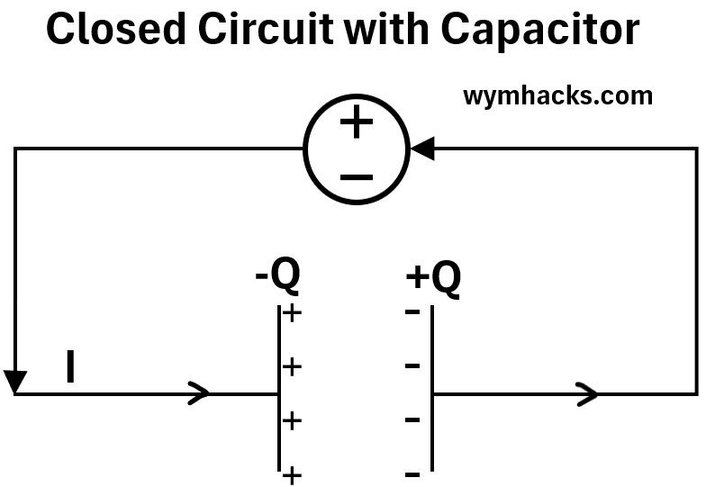
Consider a closed electric circuit with a charging parallel plate capacitor.
Picture 1 : Closed Electric Circuit with Parallel Plate Capacitor
Assume the following:
- The Parallel Plate Capacitor is Ideal:
- This means the plates are flat, parallel, and their area is significantly larger than the distance between them.
- The electric field (E) between the plates is considered to be uniform and constant in direction.
- The space between the plates is a perfect vacuum or a perfect insulator (dielectric), so no conduction current across it them.
- The current is changing with time allowing the capacitor to charge with its plates changing with time
Ampère’s Law
We know from Ampère’s law that a magnetic field will be generated around a current carrying wire. (See my post: Biot-Savart Law and Ampère’s Law)
(1) ∮B̄•dL̄ = μ0Ienc ; Ampère’s Circuital Law
Ampère’s law states that the Path Integral of B̄•dL̄ on a closed curve is equal to μ0 times the net enclosed current passing through a surface defined by the curve.
- ∮ is a closed line integral.
- i.e. summing up the contributions of the magnetic field along a complete, closed path, known as an Amperian loop.
- The integral path starts and ends at the same point.
- B̄ = Magnetic Field
- This is the magnetic field vector.
- B represents the magnitude and direction of the magnetic field at every point along the Amperian loop.
- Its SI unit is the tesla (T).
- dL̄ = Infinitesimal Line Element
- This is a small, infinitesimal vector segment of the closed loop.
- It points in the direction of the integration along the loop.
- Its SI unit is the meter (m).
- The dot product B̄•dL̄ calculates the component of the magnetic field that is parallel to the path element.
∮B̄•dL̄ ; This term is called the circulation of the magnetic field.
μ0 = Permeability of Free Space.
- A constant that represents the ability of a vacuum to support the formation of a magnetic field.
- Its value is approximately 4π×10 −7 T⋅m/A.
- Ienc = Enclosed Current:
- This is the net electric current that passes through the surface defined by the closed Amperian loop.
- It is a scalar quantity, and its SI unit is the ampere (A).
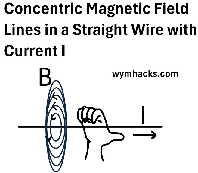
Direction of Magnetic Field
Just for completeness, let’s remember that the the direction of B is determined using the Right Hand Rule.
For our set up, B is coming out of the page.
Picture 2 : Direction of B According to the Right Hand Rule
Ampère’s Law Applied to a Flat Circular Surface Around a Conducting Wire
Let’s apply Ampère’s law to the red colored circular surface (flat disk) shown in the picture below.
Picture 3 : Closed Electric Circuit with Parallel Plate Capacitor (Flat Disk Space)
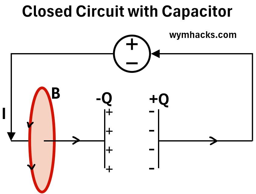
We get:
∮B̄•dL̄ = μ0Ienc
This means the magnetic field around the flat disk is proportional to the conduction current (Ienc) passing through the surface enclosed by that flat disk.
Ienc is the current passing through this surface. We can call this the conduction current IC.
So, Ampère’s Law correctly gives:
(2) ∮B̄•dL̄ = μ0IC ; Wire With Current Through A Flat Disk Surface
Ampère’s Law Applied to Cylindrical Space Around Conducting Wire and a Capacitor Plate
Now, lets expand the ‘computational’ surface from a flat disk to a cylinder.
This cylinder encompasses the wire all the way to the gap between the capacitor plates.
The only open space is the left hand side of the cylinder which is highlighted in red.
Picture 4 : Closed Electric Circuit with Parallel Plate Capacitor (Cylindrical Space)
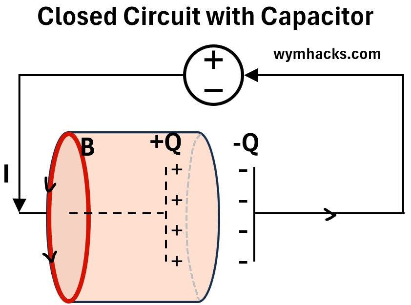
Let’s be clear on what we’ve done and what it implies:
- We took our original flat disk computational space and expanded it as a cylinder
- The surface is enclosed everywhere except on the left hand side.
This means that the original flat disk and the expanded cylindrical space both share the exact same surface boundary.
- ..upon which the integration is being done.
This means the line integral of the magnetic field ∮B̄•dL̄ should be the same as it was for the ‘flat disk” surface example.
Is it?
Well,
- we have current coming in the wire all the way to the capacitor plate,
- but there is no current coming out through any surface (remember, there is no current between the plates)
So, all the conducting and charge holding material is inside the surface of our cylinder and there is NO conduction current through this surface.
According to Ampère’s Law, the enclosed current is zero, so
∮B̄•dL̄ = μ0Ienc = 0
This creates a paradox: the integral of the magnetic field should be the same for both surfaces because they share the same boundary loop.
Ampère’s Circuital Law gives two different results, meaning it is incomplete.
So, we eventually learned that Ampere’s Circuital Law works perfectly for static (non-time-varying) magnetic fields and currents, but it fails in situations where either the electric field or current is changing over time.
The Solution
James Clerk Maxwell’s addition of the “displacement current” term to this equation corrected this flaw, leading to the complete Ampère-Maxwell law, one of the four fundamental Maxwell’s Equations.
Let’s redraw Picture 4 showing more about what is happening in the capacitor.
Picture 5 : Closed Electric Circuit with Parallel Plate Capacitor (Cylindrical Space)
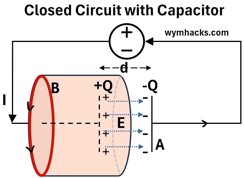
An electric field E is being generated across the parallel plates.
- From an energy balance point of view, the picture makes more sense.
- i.e. I have this current coming “in” but I also have this electrical field going “out”.
- An energy balance is being satisfied here and that is the way the world works (what comes in must come out assuming no internal consumption or generation is happening).
Recall from my Capacitance post that for two charged plates in a vacuum or air:
(3) Q/V = C = A/(4kπd) ;Parallel Plate Capacitor
(4) Q/V = C = (Aε0)/d ;Parallel Plate Capacitor
Where
- Q = Charge on each plate
- C = Capacitance and has units of Farad.
- A = Area of one of plates
- d = distance between plates
- ε0= 1/[4kπ]
- k = 1/(4πε0) = coulomb’s constant = 8.99 x 10⁹ N⋅m²/C²
- ε0 = electric constant = electric permittivity of free space (i.e. a vacuum)
- ε0 = 8.85 x 10⁻¹² C²/N⋅m² (or F/m).
Re-arrange (4)
(5) Q = VC = V(Aε0)/d
We know Voltage across the capacitor is Ed (see my Capacitance post)
(6) V = Ed ; Voltage across a Parallel Plate Capacitor
- E = Electric field in the capacitor
- d = Distance between capacitor plates
Substitute (6) into (5):
(7) Q = Ed(Aε0)/d = ε0AE
Maxwell reasoned that a changing electric field must also act as a source for a magnetic field.
Consider the charging capacitor from picture 5.
The current in the wire is the rate of change of charge on the plate:
(8) IC = dQ/dt
So, take the derivative of Q (see equation 7) with respect to time:
(9) IC = dQ/dt = d/dt [ε0AE] = (ε0A)dE/dt
Ok, we need to remember what the electric flux is (read my post Gauss’s Law for Electric Fields )
(10) ΦE = Electric Flux = (E)(A) ; Uniform E and Flat Surface Perpendicular to E
or
(11) E = ΦE/A
Substitute (11) into (9) to get
(10) IC = dQ/dt = (ε0)dΦE/dt ; Displacement Current
This result shows that the conduction current in the wire is exactly equal to the rate of change of the electric flux in the capacitor gap. This is the displacement current that Maxwell hypothesized.
Maxwell called this the displacement current, but understand that although it has units of current it is not physically a current (there is no current across the plates).
Ok, lets see if we can put this all together.
General Form of Ampère’s Law = Ampère-Maxwell Law
We’ve shown that Ampère’s Circuital law is
(1) ∮B̄•dL̄ = μ0Ienc ; Ampère’s Circuital Law
This law works for steady current situations.
We can use it for calculating magnetic fields in highly symmetric situations, such as around a long, straight wire or inside a solenoid.
However, it’s incomplete because it fails in situations with time-varying electric fields, like in a charging capacitor.
Maxwell’s addition of the displacement current term resolved this inconsistency.
Maxwell’s corrected and always true version of Ampère’s Law is
(11a) ∮B̄•dL̄ = μ0Ienc + (μ0)(ε0)dΦE/dt ; Ampère-Maxwell Law (Integral Form)
or if we substitute for the general definition of ΦE = ∫Ē•dĀ (see my post: Gauss’s Law for Electric Fields )
we get,
(12) ∮B̄•dL̄ = μ0Ienc + (μ0)(ε0)d/dt(∫Ē•dĀ) ; Ampère-Maxwell Law (integral Form)
∮ is a closed line integral.
- i.e. summing up the contributions of the magnetic field along a complete, closed path, known as an Amperian loop.
- The integral path starts and ends at the same point.
B̄ = Magnetic Field
- This is the magnetic field vector.
- B represents the magnitude and direction of the magnetic field at every point along the Amperian loop.
- Its SI unit is the tesla (T).
dL̄ = Infinitesimal Line Element
- This is a small, infinitesimal vector segment of the closed loop.
- It points in the direction of the integration along the loop.
- Its SI unit is the meter (m).
The dot product B̄•dL̄ calculates the component of the magnetic field that is parallel to the path element.
∮B̄•dL̄ ; This term is called the circulation of the magnetic field.
μ0 = Permeability of Free Space.
- A constant that represents the ability of a vacuum to support the formation of a magnetic field.
- Its value is approximately 4π×10 −7 T⋅m/A.
ε0= 1/[4kπ]
ε0 = electric constant = electric permittivity of free space (i.e. a vacuum)
ε0 = 8.85 x 10⁻¹² C²/N⋅m² (or F/m).
Ienc = Enclosed Current:
- This is the net electric current that passes through the surface defined by the closed Amperian loop.
- It is a scalar quantity, and its SI unit is the ampere (A).
ΦE = ∫Ē•dĀ = Electric Flux = a measure of the “flow” of an electric field through a given surface.
- Ē•dĀ = dot product of the electric field vector and the infinitesimal area vector.
- dΦE/dt = is the rate of change of the electric flux over time
See my article (Maxwell Equations: From Integral to Differential Forms) to learn how we can express (11a) in differential form as
(11b) ∇xB̄ = μ0 (J̅ + ε0∂Ē/∂t) ; Ampère-Maxwell Law; Differential Form
This equation shows that the “curl” (rotation) of the magnetic field at a point is caused by
- the local Current Density J and
- the local rate of change of the electric field: the term ε0∂Ē/∂t is called the Displacement Current.
Some people call this equation the “General Form of Ampère’s Law” but I wouldn’t.
James Clerk Maxwell, derived the Ampère – Maxwell equation by combining Gauss’s Law for Electric Fields and the continuity equation (see Appendix I for the derivation).
By doing this, he accomplished two amazing scientific feats
- He corrected Ampère’s Law so that it is always true but also
- predicted the existence of electromagnetic waves traveling at the speed of light. (see my post: From Maxwell’s Equations to The Wave Equation)
So, he needs his name in the equation!
The Ampère-Maxwell law can also be expressed in terms of conduction and displacement currents.
(13) ∮B̄•dL̄ = μ0IC + μ0ID ; Ampère-Maxwell Law
IC= Conduction current = the flow of electric charge (typically electrons) through a material.
ID= Displacement current = a term introduced by Maxwell to account for a changing electric field.
IT IS NOT A REAL CURRENT.
It has the same effect as a conduction current—it produces a magnetic field—but it exists even in a vacuum where no charges are moving
So, the Ampère-Maxwell law solves the paradox we thought we had in our closed-circuit-with-capacitor setup:
- For the flat surface, the conduction current term is non-zero, while the displacement current term is zero (as there’s no changing electric field to speak of in the wire).
- For the cylindrical surface, the conduction current is zero, but the displacement current term is non-zero and equal in magnitude to the conduction current of the flat surface.
- Both surfaces now give the same, consistent result.