Flux
In physics, flux (from Latin “fluxus” = flow) is the measure of how much of a vector field passes through a given surface.
Flux Using Air as an Example
Take a look at the picture below of air flowing through different windows (bounded surfaces).
Picture: Air Flux Example
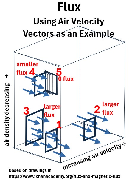
The amount of air flowing through these windows at any moment is the air flux through these “surfaces”.
In the example, the air density decreases with elevation and the air velocity increases from left to right as shown in the picture above.
Using Window 1 as a reference point,
- Window 1, perpendicular to the air flow, will have a certain amount of air flux going through it
- Shifting the same size window to the right (Window 2) will result in a larger flux (higher velocity)
- Expanding the area of the Window (Window 3) will also increase the flux.
- Elevating Window 1 to Window 4, even though its the same size , will have a lower flux (less dense, fewer particles)
- Rotating window 4 on its vertical axis through various positions all the way to a parallel position relative to the air flow (Window 5)
- Reduces the effective area through which the air can flow, thus reducing the flux
- Ultimately, when the window is parallel to the flow (Window 5) it will be zero.
Similarly, in physics, flux is a way to quantify the “flow” of things that may not be a physical substance, such as an electric or magnetic field.
The amount of flux depends on three factors:
- The strength of the field (e.g., how fast the river is flowing or how strong the electric field is).
- The area of the surface (e.g., the size of the net or window a vector field flows through).
- The orientation of the surface relative to the field.
- Flux is at its maximum when the surface is perpendicular to the field
- and zero when it’s parallel to the field.
Flux in Physics
The most common types of flux in physics are electric flux and magnetic flux.
Electric Flux
Electric flux, ΦE , is the measure of an electric field passing through a surface.
It helps us understand the relationship between electric charges and the electric fields they produce.
Magnetic Flux
Magnetic flux , ΦB , is the measure of a magnetic field passing through a surface.
It’s crucial for understanding how magnetic fields generate electric currents.
We’ll cover these is in detail in the following sections.
Electric Flux and Gauss’s Law for Electric Fields
Check out my dedicated article on this topic: Gauss’s Law for Electric Fields
Note, in a later section, we will make an analogous description for Gauss’s Law for Magnetic Fields.
Gauss’s Law for electric fields is a fundamental principle in electromagnetism that relates the distribution of electric charge to the electric field it produces.
It states that the total electric flux out of any closed surface is directly proportional to the total electric charge enclosed within that surface.
- The term flux is a measure of “how much of something passes through a given surface.”
- For electric flux, that “something” is the electric field E
Equation for Electric Flux Through a Surface
Please refer to my post Gauss’s Law for Electric Fields for more details and a derivation of the equation presented in this section.
Consider a uniform Electric Field as drawn in the picture below. E passes through a flat window of area A which has a perpendicular component Ap.
Picture: Side View; Uniform E Field through Flat Surface
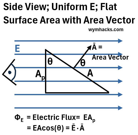
The area vector , shown as the arrow emanating from surface A, represents the area of A and is perpendicular to A.
Note that in order to calculate Ap using basic trigonometry (see my article ‘Geometry and Trig Rules’), we need to know θ (because Ap = Acos(θ))
And , crucially, note that θ will always equal the angle the area vector makes with the E field vector.
So, this allows us to restate the electric flux for a uniform E and a flat surface as:
ΦE = Electric Flux = (E)(Ap) =EAcos(θ) =Ē•Ā ; for Uniform E and Flat Surface
where,
-
ΦE = Electric Flux (units: (N/C)m2)
- Ap (units: m2) = Perpendicular component of A that the electric field passes through.
- E = The electric field (units: N/C)
- Ē•Ā = dot product of the electric field vector and the area vector.
- θ = angle between area vector and E vector
For any E through any surface we can restate the equation as the integral of E times infinitesimal areas.
ΦE = Electric Flux = ∫EdAcos(θ) =∫Ē•dĀ for any E for any surface
where, we now have a general expression for the electric flux through any surface.
Gauss’s Law for Electric Fields
Consider a spherical area (with radius R) around a central positive electric charge.
Flux E in a Sphere Containing a Central Charge
Picture: Electric Flux from a Sphere with Positive Charge at Center.
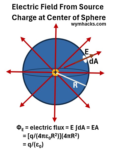
We want to calculate the electric flux for E through this sphere.
Let’s start with a general form of the electric flux equation (see my post Gauss’s Law for Electric Fields) for more on its formulation)
ΦE = Electric Flux =∫EdAp = ∫EdAcos(θ) =∫Ē•dĀ for any E for any flat surface
For everywhere on the surface dA,
- the surface is perpendicular to the radius R which is parallel to E.
- So, θ = 0 and cos(0) = 1
- and E is constant so
ΦE = E ∫dA = EA
From Coulomb’s Law we know that
- E = Fe/q2(test) = kq1(source)/R2 and
- k = 1/(4πε0)
Substituting into our flux equation we get,
ΦE = [q/(4πε0R2)](4πR2)
ΦE = q/ε0
Where q is (+) for a positive charge and q is (-) for a negative charge.
What Happens if we Adjust The Radius R?
Nothing. There is no R term in the spherical Flux equation.
Flux is independent of size due to inverse square law characteristic of Coulomb’s law.
What Happens if We Move The Charge Off Center in the Sphere?
Even though E and θ are no longer constant, the flux will remain the same (see Appendix 2 in my Gauss’s Law for Electric Fields post for the proof).
What Happens if We Have a Charge in some Non-Uniform Surface?
As long as the surface is closed, it doesn’t matter. Flux is the same. The proof provided in Appendix 2 in my Gauss’s Law for Electric Fields…post is independent of shape.
What Happens if We Have More Than One Charge Enclosed in the Area?
Just sum up the charges i.e. Φ = Σq/ε0
What Happens if We Have Charges Outside the Surface?
Charges outside a closed surface do not contribute to the net electric flux through that surface.
So we began with a specific scenario of a Sphere but ended up with the most general form of the equation for the E flux.
∮Ē•dĀ = qenclosed/ε0 ; Gauss’s Law for Electric Fields ; Integral Form
- Where q is the charge enclosed in the surface (any closed surface)
- This equation is called Gauss’s Law for Electric Fields
- It is the integral form of one of the four Maxwell Equations.
Differential Form of Gauss’s Law for Electric Fields
In my post From Maxwell’s Equations to The Wave Equation, I describe the differential form of Gauss’s Law for Electric Fields and the mathematical language behind it.
Also refer to my article: Maxwell Equations; From Integral to Differential Forms where I derive the differential form from the integral from (using the Gauss’s Divergence Theorem and Stokes’s Theorem).
∇⋅Ē = ρ/ε0 = 4πkρ ; Gauss’s Law for Electric Fields ; Differential Form
Variable Descriptions
- ∮ = the surface integral over a closed surface
- ∇⋅ = Divergence Operator where ∇ = nabla or del.
- Ē = Electric Vector Field
- ρ = charge density = charge/volume = q/V
- ε0 = electric permittivity of free space
- It is a fundamental physical constant that represents the ability of a vacuum to permit electric field lines.
- ε0 = 8.854×10⁻¹² Farads per meter (F/m)
- k = Coulomb’s Constant = electrostatic constant = 1/(4π ε0) ≈8.99×10⁹ N⋅m2/C2
- μ0 = magnetic permeability of free space = magnetic constant = 4π×10-7 H/m (Henrys per meter).
- It is a fundamental physical constant that describes how a vacuum responds to a magnetic field.
- c = 1/sqrt(μ0ε0) = speed of light = 299,792,458 m/s
- π = pi = 3.1415..
Gauss’s Law for Electric Fields Description
Gauss’s Law for Electric Fields states that electric charges q give rise to electric fields E in a direction based on the sign of the electric charge.
From the differential form the law tells us:
- a charge q (where ρ = charge/volume) creates an electric field E.
- electric fields E act in a divergent way (∇⋅E) , meaning they are flowing outward or inward.
- An electric charge acts as a source or sync for the electric field E.
From the integral form the law tells us:
- The electric flux emanating from a close surface is equal to the charge enclosed by that surface.
- The flux of a vector field is the amount of the field passing through the closed surface
Summary: Gauss’s Law for Electric Fields
- the total electric field passing through that surface depends only on the amount of charge inside it.
- Charges outside the surface do not contribute to the net flux.
- This law is one of Maxwell’s four equations of electromagnetism and is a powerful tool for calculating electric fields.
Magnets and Magnetic Fields
Magnets
A magnet is a material or object that produces a magnetic field, causing it to attract or repel other objects made of iron or other metals.
The Greek term “magnētis lithos”, meaning “Magnesian stone”, refers to Magnesia, a region in ancient Anatolia (modern-day Turkey), where lodestones (naturally magnetized iron ore) were found.
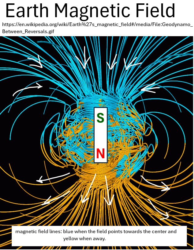
The earth’s core is essentially a magnet that generates a magnetic field.
- Liquid metal in the outer core of earth
- generates electric currents
- a spinning earth with electric currents creates a large self sustaining magnetic field
Why Does Earth Have A Magnetic Field?
Magnetic Properties
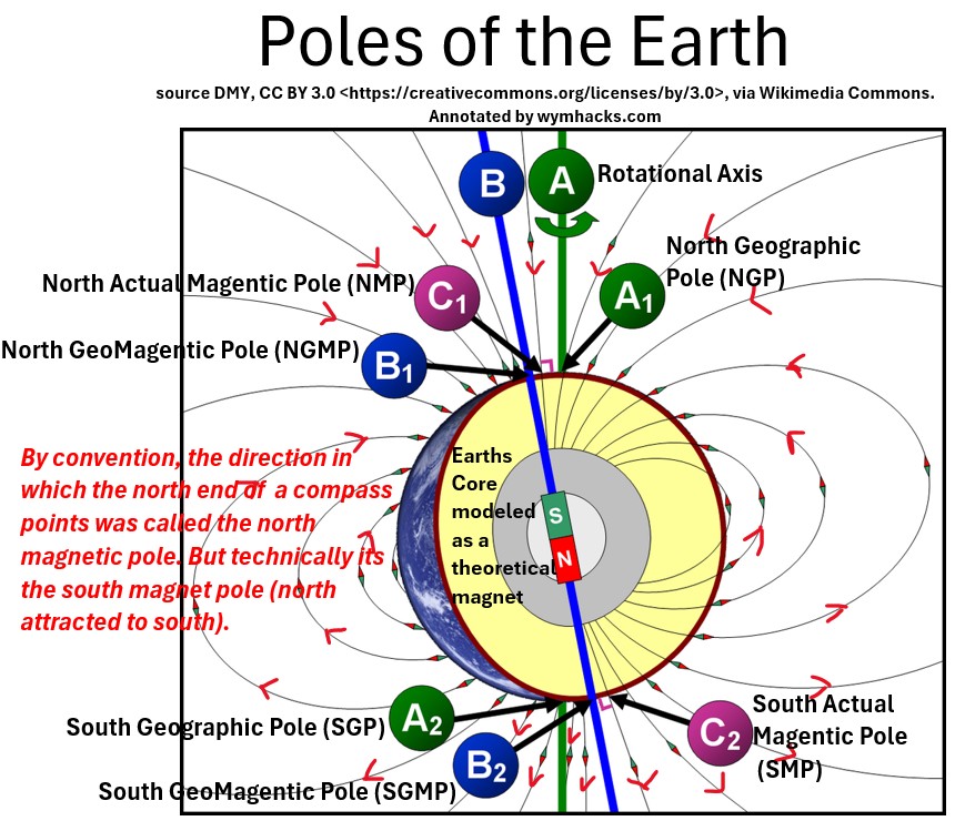
- Magnets have two poles (A north pole and a south pole).
- The north pole (for example in a compass) will point towards the south magnetic pole of earth
- By convention we called the south magnetic pole the north magnetic pole. I know. Kind of stupid.
- See the Poles of the Earth picture below.
- The Geomagnetic Poles are theoretical poles aligned with a theoretical magnet created by the earths core.
- The Magnetic Poles are poles that move around (they are the actual poles).
- By convention, the Geomagnetic North and South Poles are on the same sides as the Geographic North and South Poles
- By convention, the Magnetic North and South Poles are on the same sides as the Geographic North and South Poles
- Technically, the north and south magnetic poles are on opposite sides of the Geographic poles
- Magnets generate a magnetic field.
- Magnetic fields move from the north pole to the south pole.
Picture: Magnetic Field Lines in a Magnet
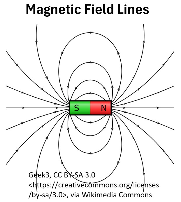
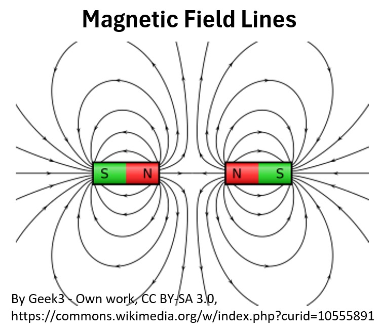
- Opposite poles attract and like poles repel each other.
Picture: Magnetic Field Lines of 2 Magnets – N to N Ends (Repulsion)
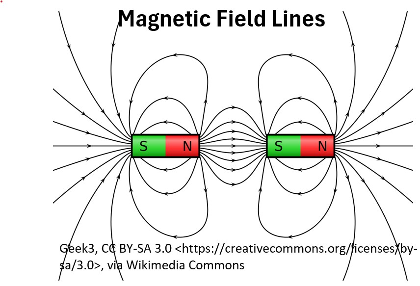
Picture: Magnetic Field Lines of 2 Magnets – N to S Ends (Attraction)
- Magnets always align in a north/south direction (always aligns with earths magnetic field)
- Magnetic poles ALWAYS exist in pairs (can’t have monopoles)
- A single charge can produce an electric field (an example of a monopole).
- The magnetic field is strongest at the poles
Picture: Poles of the Earth
What Causes Magnetism?
Magnetism is a manifestation of the electromagnetic force, one of the four fundamental forces of nature.
- It arises from the movement and alignment of charged particles, particularly electrons, both at the atomic and macroscopic levels
- This is true from the smallest subatomic particles to large-scale phenomena like Earth’s magnetic field.
Electron Spin
Electrons have a property called “spin,” which makes them behave like tiny basic magnets.
For most materials, these electron spins are randomly oriented resulting in no net magnetism.
But, in certain materials like iron, nickel, and cobalt (ferromagnetic materials),
- the spins of electrons in adjacent atoms spontaneously align in the same direction.
- This alignment creates a cumulative magnetic field that can be observed (i.e. a permanent magnet).
Electron Orbital Motion
Electrons also rotate around the nucleus of an atom.
- These moving electric charges generate a tiny magnetic field.
Electric Currents
In a later section we will see that an electric current produces a magnetic field around it.
- This is the principle behind electromagnets, electric motors, and generators.
- The strength and direction of the magnetic field depend on the magnitude and direction of the current.
Ok, we now know a little about magnetism.
Also, you might want to watch these great videos:
Magnetic Flux and Gauss’s Law for Magnetic Fields
This part is structured like the section on “Electric Flux and Gauss’s Law for Electric Fields”
Let’s remember what “flux” means in physics.
- The term flux is a measure of “how much of something passes through a given surface.”
- For Electric Flux, that “something” is the electric field E and for a magnetic flux, that “something” is the magnetic field B.
- The Magnetic Flux, ΦB (Phi), is the measure of a magnetic field passing through a surface.
Gauss’s Law for Magnetic Fields states that the net magnetic flux through any closed surface is always zero.
This is a fundamental principle of electromagnetism and one of Maxwell’s equations.
- The law’s most significant implication is that magnetic monopoles do not exist.
- Unlike electric charges, magnetic poles must always come in pairs (north and south).
- Magnetic field lines never start or end at a point; they always form continuous, closed loops.
Equation for Magnetic Flux Through a Surface
Please refer to my post Gauss’s Law for Electric Fields for more details.
- Although the post develops the Electric Flux equation, the same methodology and logic would be used to derive the magnetic flux equation through a flat surface.
Consider a uniform Magnetic Field as drawn in the picture below. B passes through a flat window of area A which has a perpendicular component Ap.
Picture: Side View; Uniform B Field through Flat Surface
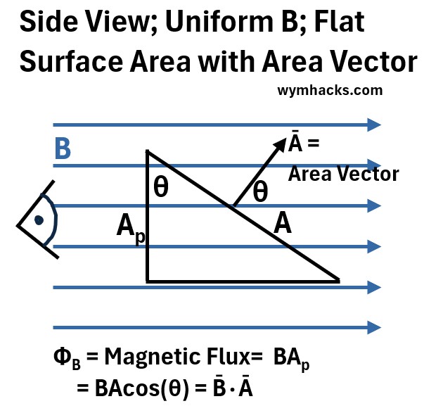
The area vector , shown as the arrow emanating from surface A, represents the area of A and is perpendicular to A.
- Note that in order to calculate Ap using basic trigonometry, we need to know θ (because Ap = Acos(θ))
- And , crucially, note that θ will always equal the angle the area vector makes with the B field vector.
The magnetic flux for a uniform B and a flat surface is:
ΦB = Magnetic Flux = (B)(Ap) =BAcos(θ) =B̄•Ā ; for Uniform B and Flat Surface
where,
- ΦB = Magnetic Flux (units: (N/C)m2)
- Ap (units: m2) = Perpendicular component of A that the Magnetic field passes through.
- B = The Magnetic field (units: N/C)
- B̄•Ā = dot product of the Magnetic field vector and the area vector.
- θ = angle between area vector and B vector
For any B through any surface we can restate the equation as the integral of B times infinitesimal areas.
ΦB = Magnetic Flux = ∫BdAcos(θ) =∫B̄•dĀ for any B for any surface
where, we now have a general expression for the magnetic flux through any surface
For magnetic flux through a closed surface, we’ll see that this expression will always equal zero.
These expressions are utilized in Faraday’s law (see Faraday’s Law section).
Magnet Behavior
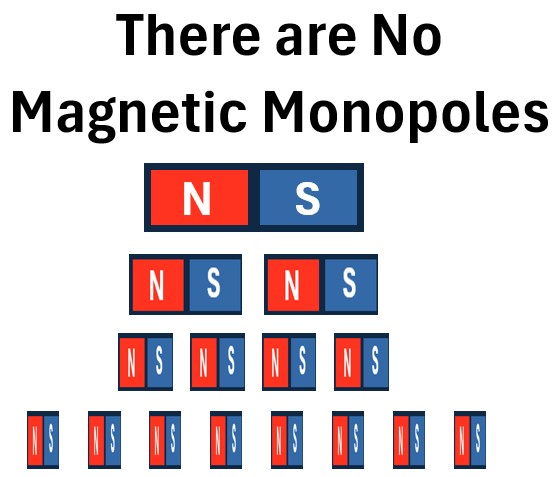
If you take a magnet and keep breaking it into two pieces, even to an atomic level, you will always end up with magnets that have both a north and a south pole.
That is, unlike electric charges, magnets
- are always magnetic dipoles.
- don’t exist as monopoles (We haven’t found them yet.)
Picture: Splitting A Magnet Always Gives You More Magnets
Magnetic Flux Behavior
Let’s do a simple visual experiment where we put electric or magnetic fields in a sphere and see if we can make some observations about the flux and the enclosed field in relation to the spherical surface.
Consider the electric flux of a charge in an enclosed surface.
Picture: Electric Charge in a Close Surface
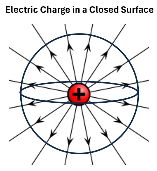
Gauss’s Law for Electric Fields tells us that a closed surface integral of the dot produce of E and A will equal the amount of charge enclosed in that surface divided by epsilon naught or:
∮Ē•dĀ = qenclosed/ε0 ; Gauss’s Law for Electric Fields ; Integral Form
- Where q is the charge enclosed in the surface (any closed surface)
- This equation is called Gauss’s Law for Electric Fields
- It is the integral form of one of the four Maxwell Equations.
In the picture below we now put an electric dipole (a plus and a minus electric charge) into a sphere.
Picture: Electric Dipole in a Close Surface
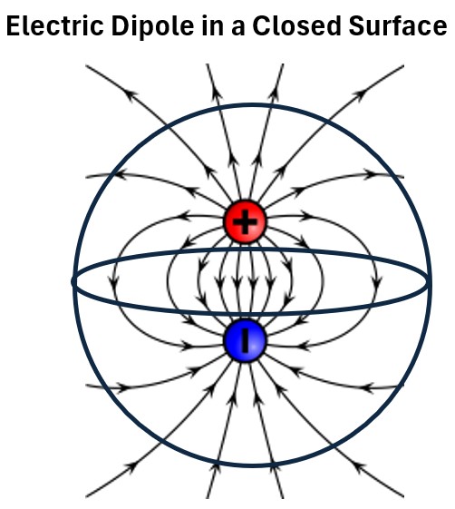
The number of fields leaving will equal the number of fields entering, so the E flux is zero and the enclosed charge is zero.
A very similar scenario will be a magnet (a magnetic dipole) in a sphere shown below.
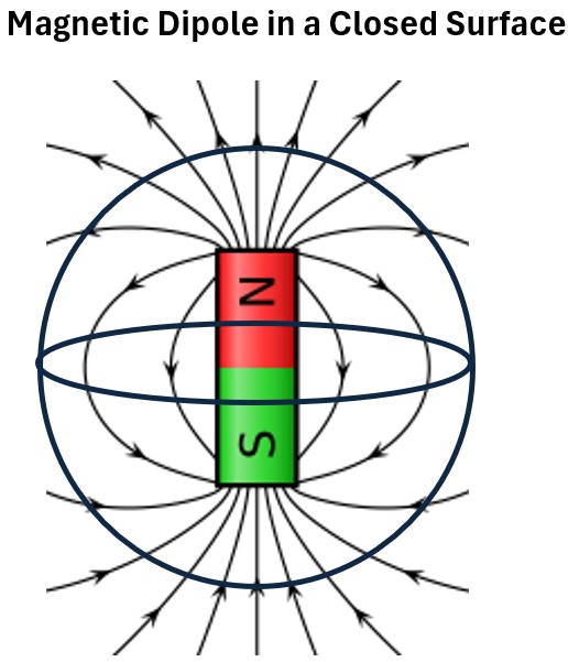
We get the same outcome as we did for an electric dipole: Zero B flux and Zero B enclosed.
Now, consider a magnet adjacent to but outside our spherical reference point, as shown below.
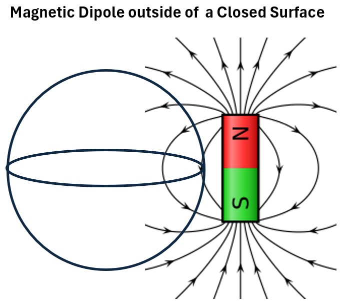
The B lines offset each other into and out of the spherical space so once again: Zero B flux and Zero B enclosed.
Finally, what happens if we put half the magnet into the spherical space.
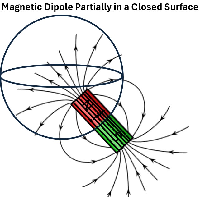
If you remember that the magnetic field lines are also running through the magnet’s internals, then all the B lines (relative to the spherical space) offset each other.
So, once again, the magnetic flux is zero.
Gauss’s Law for Magnetic Fields
We are ready to state Gauss’s Law for Magnetic Fields:
∮B̄•dĀ = 0 ; Gauss’s Law for Magnetic Fields ; Integral Form
- A closed surface integral of the dot product of B and A will equal zero.
- The net magnetic flux through any closed surface is always zero.
- It is the integral form of one of the four Maxwell Equations.
- Magnetic monopoles do not exist.
- Magnetic field lines never start or end at a point; they always form continuous, closed loops.
This equation can be expressed in its differential form as well.
See my post Maxwell Equations; From Integral to Differential Forms to see how to do this.
(∇⋅B̄) = 0 ; Gauss’s Law for Magnetic Fields ; Differential Form
This equation says, in magnetism, because the divergence is always zero, you can never have a source or a sink.
This leads to two big real-world conclusions:
- The Dipole Rule: Magnets always come in pairs (North and South).
- If you snap a bar magnet in half, you don’t get a North piece and a South piece; you get two smaller magnets, each with its own North and South pole.
- Continuous Loops: Magnetic field lines don’t start or stop anywhere; they form continuous, closed loops.
- Every line that leaves the North pole must return to the South pole.
Orsted! Current Creates a Magnetic Field (I → B)
An electric current produces a magnetic field around it (discovered by H.C. Orsted)
Orsted (1820)
In 1820, experiments done by Danish physicist Hans Christian Orsted showed a link between electricity and magnetism.
Many accounts on the web suggest his discovery was accidental.
According to descriptions in the book “Faraday , Maxwell, and the Electromagnetic Field by Forbes and Mahon” , I would not use the word accidental.
- Orsted wanted to know what effects if any a wire with current through it (current and resultant heat and light)
- would have on a compass placed near it.
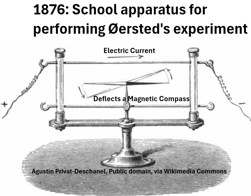
He did this during a live lecture. When he connected the battery, the compass feebly twitched.
The experiment had very little effect on the audience.
Three months later Orsted modified the apparatus to pass more current, and this time
- the compass needle took on a new fixed position which
- was at a right angle to the wire.
This and subsequent experiments led to the following observations
- As the current increases, so does the strength of the magnetic field (I ↑, B ↑)
- The strength of the magnetic field decreases with distance from the wire (Distance ↑, B ↓)
- The magnetic field forms concentric circles around a straight wire (at all distances)
- The direction of the field depends on the direction of the current.
This discovery was revolutionary because, prior to this, electricity and magnetism were considered separate phenomena.
Orsted’s work laid the foundation for the entire field of electromagnetism.
Use the Right Hand Thumb (Grip or Curl) rule to determine the direction of the magnetic field created by a current.
Picture: The Right Hand Thumb (Grip, Curl) Rule
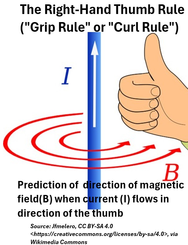
With your right hand in a clenched thumbs up position,
- point your thumb in the direction of current flow I.
- Your clenched fingers indicated the direction/path of the magnetic field B.
- Right hand thumb rule – KhanAcademy
See the picture below for an example of how to apply it.
Picture: Current Flowing in a Wire Produces a Magnetic Field
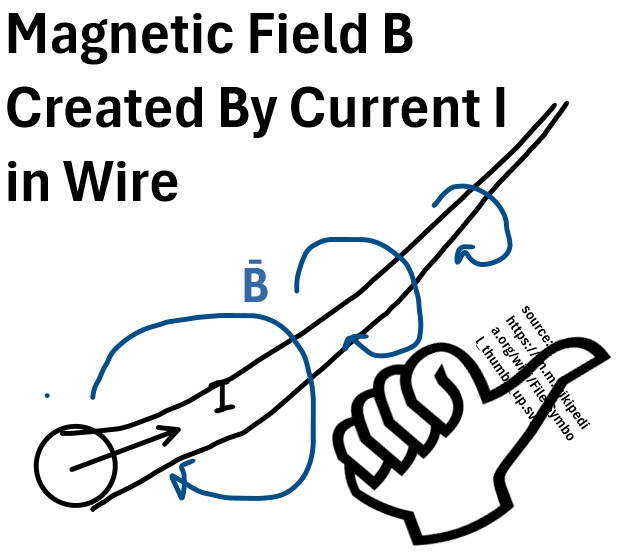
See my post: Current and Magnetic Field Right Hand Rule Examples for more examples.
Also refer to this great video: Magnetic Fields around Wires, Coils, and Poles of Bar Magnets – Dr. Pierce’s Physics & Math
Magnetic Force on a Current Carrying Wire
We learned in a previous section that a wire carrying current creates a magnetic field.
This magnetic field exerts a force on a magnet carrying compass.
Newton’s Third Law says that “for every action, there is an equal and opposite reaction.”
So we would expect an magnetic force to be exerted on a current carrying wire in a magnetic field.
The equation we need to compute this is the equation we introduced in the previous section: the Lorentz Force Equation.
The Lorentz Force Equation
F̅ = F̅e + F̅B
or
F̅ = qE̅ + q(v̅ x B̅)
or
F̅ = q(E̅ + (v̅ x B̅)) ; The Lorentz Force Equation
where
- F̅ = Total Force. The Lorentz Force
- F̅B = Force on charge q by magnetic field B
- F̅e = Force on charge q by electric field E
- q = charge
- v = velocity of charge
- E̅ = electric field
- B̅ = Magnetic Field
- θ = Angle between velocity and direction of B
We want to convert this equation into a form showing current and length.
Lets assume we just want to look at the magnetic field B effects (No E).
Then
F̅B = q(v̅ x B̅) ; Magnetic Component of the Lorentz Force
Let v̅ = distance/time = L̅/t
Substitute for v̅ :
F̅B = q/t(L̅ x B̅) ; Magnetic Component of the Lorentz Force
But q/t is the current I so:
F̅B = I(L̅ x B̅) ; Magnetic Component of the Lorentz Force
which can also be expressed in magnitude form (remember your vector calculus rules):
FB= ILBsinθ ; Magnitude of Magnetic Component of the Lorentz Force (uniform B, straight wire, constant I)
where
- F̅B = magnetic force acting on wire
- I = constant current flowing through wire (in Amperes)
- L̅ = length or distance of wire segment inside magnetic field
- B̅ = magnetic field (in Tesla)
- F, L, B = magnitudes of F, L, and B
- θ = angle between L̅ and B̅ vectors
Picture: Magnetic Force on a Current Carrying Wire
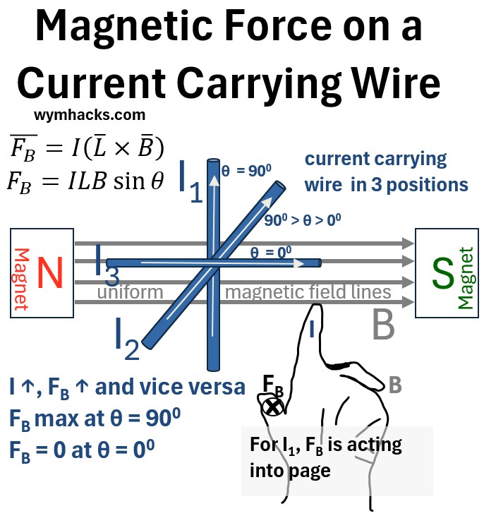
This setup will have the following properties:
- The wire in position I1 (90 degrees to the direction of B) will have the maximum magnetic force F acting on it
- The wire in position I3 will have zero F acting on it (it is parallel to the magnetic field B)
- Force will increase with increasing current I
- The direction of F depends on the direction of B and I
- For I1, the direction of F is into the page and perpendicular to B and I.
- The direction is determined by the cross product right hand rule
- Index finger pointed at L (which is in direction of I)
- Middle finger pointed at B
- Thumb pointed at F
See my post Magnetic Force on a Current Carrying Wire for an example that uses this equation.
This is a very important concept in physics.
A magnetic field’s ability to exert a force on a current-carrying wire has enormously important industrial applications.
It forms the fundamental principle behind many technologies like:
- Electric Motors: Magnetic fields exert torque on current-carrying coils, causing continuous rotational motion.
- Loudspeakers: A current-carrying coil attached to a cone moves within a magnetic field, producing sound.
- Galvanometers/Ammeters: Current in a coil within a magnetic field produces a torque, deflecting a needle to measure current.
- Relays: A current in a coil creates an electromagnet that pulls an armature to open or close contacts.
- Magnetic Levitation (Maglev) Trains: Magnetic fields lift and propel current-carrying coils on the train, or interact with currents induced in the track.
- Actuators (Solenoids): A current through a coil creates a magnetic field that pulls a ferromagnetic core or a current-carrying element, causing linear motion.
Biot Savart Law and Ampère’s Law
The Biot-Savart Law and Ampere’s Law both describe the relationship between a steady electric current and the magnetic field it produces.
- The Biot-Savart law describes the magnetic field generated by a steady electric current.
- Ampere’s law, which is derived using the Biot-Savart Law, provides a relationship between the magnetic field circulating around a closed loop and the total electric current passing through that loop.
They are analogous to Coulomb’s law and Gauss’s Law for Electric Fields (electrostatics).
You should review my post: Biot-Savart Law and Ampère’s Law for an in-depth review with derivations.
Biot-Savart Law
Consider B generated by a moving point charge i.e. B generated by a current.
Picture: B Generated by Current I Straight Wire
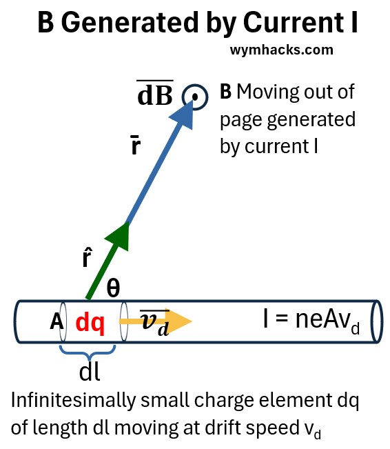
In this case we consider an infinitesimal length dl with an infinitesimal charge dq moving at a drift velocity v̄d.
And this causes an infinitesimal magnetic field dB̄ at a specific location r̄ away from the element.
We can derive the following: (Review my post: Biot-Savart Law and Ampère’s Law for an in-depth review with derivations)
dB̄ = [μ0/(4π)] (I) (dl̄xr̂)/r2 ; Differential Form of Biot-Savart Law
∫dB̄ = B̄ = [μ0/(4π)] (I) ∫ [ (dl̄xr̂)/r2 ] ; Integral Form of Biot-Savart Law
The magnitude of the vector dB̄ is dB and we know how to express it (see cross product rules):
dB = [μ0/(4π)] (I) dlsinθ/r2 ; Magnitude of the Differential Form of Biot-Savart Law
where
- I = Current in wire
- B = magnetic field
- μ0= the permeability of free space or the magnetic constant.
- μ0is a fundamental physical constant which shows how easily a magnetic field can pass through a vacuum
- μ0= 4π×10−7 Tesla-meters/Amp = Henry/meters
- v̄ (v bar) = drift velocity vector
- r = distance from q to the point at which B is being measured
- r̂ (r hat) = unit vector r
- θ = angle between v̄ (v bar) and r̂ (r hat)
- dB is the magnitude of an infinitesimally small magnetic field caused by infinitesimally small charge (current) element
- dl̄ = infinitesimal length l of charge dq
- dl̄xr̂ = |dl̄||r̂|sinθ where | | is the magnitude symbol (by definition: see Vector Math)
- |r̂| = 1 (it’s a unit vector)
B and E behave Differently
Recall the equation for the strength of an electric field caused by a point charge
E = kq/r2 ; E = strength of the electric field; k = Coulomb’s constant, q = magnitude of source charge, r = distance of E from point charge
It is structurally similar to the dB magnitude equation except for one huge difference: sinθ
For E, at a certain distance from r (anywhere) from the source charge, it is the same value.
But for dB, the strength will vary at the same r depending on the measurement point’s position relative to the charge (current) element.
- When perpendicular, dB will be maximum
- When parallel to the current element, it will be zero
Direction of B
In the drawing above , B is coming out of the page.
There are two ways to determine the direction of the magnetic field B using the right hand.
- Put your thumb in the direction of current. Curling fingers are the direction of B
- Put back of palm on dl and sweep with fingers from dl̄ to r̂. Thumb points in direction of B.
Biot Savart Law in Words
- the current,
- the length of the segment,
- the sine of the angle between the current direction and the line to the point of observation, and
- is inversely proportional to the square of the distance from the segment to that point.
The total magnetic field is found by summing (integrating) the contributions from all such small segments of the wire.
The direction of the magnetic field is determined by the right-hand rule.
Ampère’s Law
Consider a closed loop (not necessarily circular) upon which we are measuring B.
Assume the surface it bounds is being “penetrated by” multiple wires carrying currents.
Picture: B on a Closed Loop Around Multiple Wires with Current
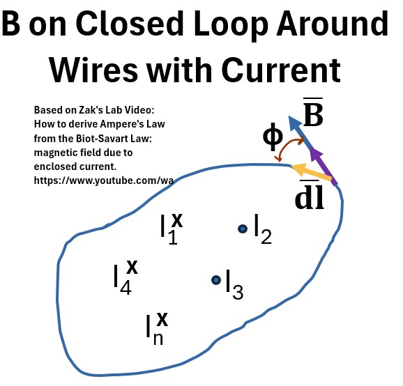
We can derive the following: (Review my post: Biot-Savart Law and Ampère’s Law for an in-depth review with derivations)
∮B̄•dl̄ = ∮B̄•dL̄ = μ0Ienc ; Ampere’s Circuital Law
It states that the Path integral of B̄⋅dl̄ on a closed curve is equal to μ0 times the net enclosed current passing through a surface defined by the curve.
note: we can also use upper case L (versus lower case l) to make the length variable more conspicuous in the expression.
where
- ∮ is a closed line integral.
- i.e. summing up the contributions of the magnetic field along a complete, closed path, known as an Amperian loop.
- The integral path starts and ends at the same point.
- B̄ = Magnetic Field
- This is the magnetic field vector.
- B represents the magnitude and direction of the magnetic field at every point along the Amperian loop.
- Its SI unit is the tesla (T).
- dl̄ = dL̄ = Infinitesimal Line Element
- This is a small, infinitesimal vector segment of the closed loop.
- It points in the direction of the integration along the loop.
- Its SI unit is the meter (m).
- The dot product B̄⋅dl̄ calculates the component of the magnetic field that is parallel to the path element.
-
∮B̄•dl̄ ; This term is called the circulation of the magnetic field.
-
μ0 = Permeability of Free Space.
- A constant that represents the ability of a vacuum to support the formation of a magnetic field.
- Its value is approximately 4π×10 −7 T⋅m/A.
- Ienc = Enclosed Current:
- This is the net electric current that passes through the surface defined by the closed Amperian loop.
- It is a scalar quantity, and its SI unit is the ampere (A).
- Currents flowing in one direction are considered positive, and those flowing in the opposite direction are considered negative, according to the right-hand rule.
Ampere’s Law in Words
Ampere’s Law states that the circulation of a magnetic field around a closed loop is directly proportional to the total electric current passing through the surface bounded by that loop.
i.e. the magnetic field strength integrated along that path (circulation) is directly related to the amount of current enclosed by the path.
The direction of the magnetic field follows the right-hand rule.
Ampere’s Law is Not Quite Complete!
Ampère’s law (or Ampère’s Circuital Law) is fundamentally incomplete because it only accounts for magnetic fields created by conduction current (moving charges).
This posed a major problem in circuits with charging capacitors, where it incorrectly predicted a zero magnetic field in the gap where no actual current flows.
James Clerk Maxwell solved this by introducing the displacement current term (∂t), which accounts for a magnetic field being generated by a time-varying electric field, thereby ensuring the law’s consistency and ultimately predicting the existence of electromagnetic waves.
I address this in detail in my post Electricity (8/11) Maxwell’s Equations when I describe the Ampère Maxwell Equation.
I also wrote a separate post about it here: Ampère Maxwell Equation
Faraday! A Changing Magnetic Field Creates Current (B → I)
A changing magnetic field can induce an electric current (discovered by Michael Faraday 1831).
Michael Faraday, in a series of experiments in 1831, discovered the phenomenon of Electromagnetic Induction.
Electromagnetic Induction occurs when
a changing magnetic field (due to a magnet or coil moving or magnetic field strength changing)
produces an electric current (due to a created electromotive force, EMF) in a conductor.
This means that
if a conductor moves through a magnetic field, or
if the magnetic field around a conductor changes,
an electric current will be induced in the conductor, provided it’s part of a closed circuit.
This principle is fundamental to how generators, transformers, and many other electrical devices work.
See my following posts for more on generators and transformers
Michael Faraday proved this principle in a series of experiments done in 1831:
the Iron Ring Experiment ,
the V-Magnet Experiment, and
The Magnet and Coil Experiment
Below is a schematic of the experimental set up for the Magnet and Coil Experiment.
Picture: Faraday Magnet and Coil Experiment 1831
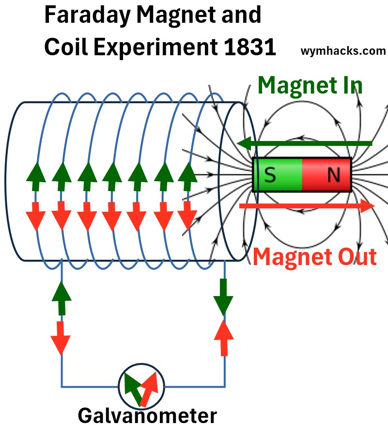
Basically,
- when a magnet was moved into and out of the coiled device,
- the Galvanometer needle swung vigorously,
- proving an current was being induced by the movement of the magnet (a changing magnetic field).
Faraday’s groundbreaking experiments provided the conceptual foundation for electromagnetic induction.
But, another 30 years would pass before James Clerk Maxwell translated them into a precise mathematical expression.
References
Learn more about Michael Faraday’s experiments in my post: Faraday’s 1831 Electromagnetic Experiments
If you want to read a really good book on Michael Faraday and his experiments (or really on electromagnetism in general), then read this one:
- Faraday, Maxwell, and the Electromagnetic Field by Nancy Forbes and Basic Mahon; 2019; By Prometheus Books
You can also review these nice electromagnetic Induction Videos:
Faraday’s Law: Flux Rule
Ok, let’s continue exploring Faraday’s law of electromagnetic induction.
Magnetic Flux
Let’s start by revisiting the definition of magnetic flux (see the magnetic flux section of this post):
Picture: Magnetic Field B and Magnetic Flux
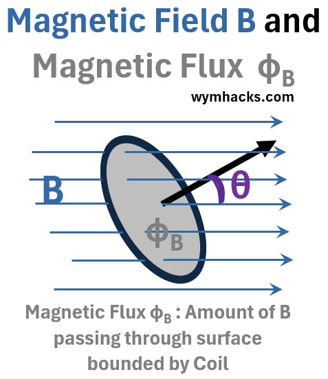
Magnetic flux , ΦB , is the measure of a magnetic field passing through a surface.
ΦB = Magnetic Flux = (B)(Ap) =BAcos(θ) = B̄•Ā ; for Uniform B and Flat Surface where
- ΦB = magnetic Flux (units: (N/C)m2)
- Ap (units: m2) = Perpendicular component of A that the magnetic field passes through.
- B = The magnetic field (units: N/C)
- B̄•Ā = dot product of the magnetic field vector and the area vector.
- θ = angle between area vector and B vector
ΦB = Magnetic Flux =∫BdAcos(θ) =∫sB̄•dĀ for any B for any surface
- For any B through any surface we can restate the equation as the surface integral ∫s of B times infinitesimal areas.
- This is a a general expression for the magnetic flux through any surface
So, what can change magnetic flux? From the equation (and the drawing) we know it is
- A change in the magnitude of B
- A change in the surface area B passes through and
- A change in the angle between B and the surface
Faraday’s Law of Electromagnetic Induction: Flux Rule
It was the Scottish physicist James Clerk Maxwell, about 30 years later, who translated Faraday’s experimental work and conceptual ideas into the precise mathematical form we use today.
The general form of Faraday’s law of induction describes how a changing magnetic field creates an electromotive force (EMF) in a circuit (i.e. electromagnetic induction):
EMF=−Nd/dt ; Faraday’s Law of Electromagnetic Induction (the Flux Rule)
or
Δt ; Faraday’s Law of Electromagnetic Induction (the Flux Rule) – Average form
where
- EMF (symbolized as ε) is the induced electromotive force (EMF).
- EMF is not really a force.
- It is a measure of the energy per unit charge, similar to voltage, that causes a current to flow in a closed circuit.
- It’s measured in Volts (V).
- The EMF is the driving potential that gets charges moving.
- N: the number of turns in the coil of wire.
- is the sum of the EMFs induced in each individual loop.
- dΦB/dt : the instantaneous rate of change of the magnetic flux through the circuit.
- ΦB : the magnetic flux
- The Negative Sign (-): this represents Lenz’s Law (more on this below).
- i.e. the direction of the induced EMF (and the resulting current) is such that it creates a magnetic field that opposes the change in magnetic flux that produced it.
- The average form of Faraday’s law of induction is used to calculate the average induced electromotive force (EMF) over a specific, finite time interval.
- You write it by replacing the differential symbols with delta symbols.
Faraday’s Law: Coil in a Magnetic Field
The picture below is a plan view of a magnetic field coming out of the page towards you (represented by the circles with dots…where you can imagine the dots to be the tips of arrows).
We’ll drop a rectangular conducting coil into this field such that its bounded surface is perpendicular to the B field.
Picture: Magnetic Field Lines With Closed Loop Conducting Wire
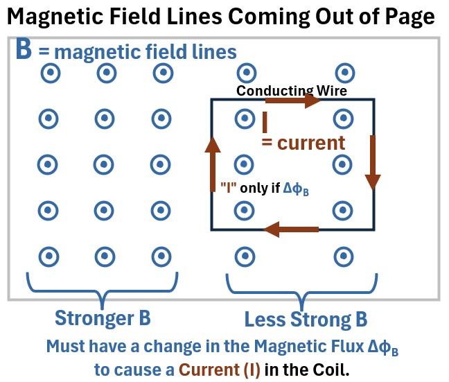
The B field is shown as having various fixed (constant) intensities based on the distance of the points from each other.
As long as the field is constant and the coil is stationary we will not see any current in this coil.
A current “flows” in the wire only if the magnetic flux changes.
So, a current I will start “flowing” in the loop if the magnetic flux changes somehow (ΔΦB > 0):
- e.g. the flux strength decreases or increase
- e.g. the conducting wire boundaries are expanded or contracted
The current I direction is shown going clockwise in the schematic. How do we know that? Read on!
References
Lenz’s Law
Induction and Lenz’s Law (The Negative Sign In Faraday’s Law)
Lets rotate the picture in the previous section so we see a side view of the coil and the magnetic field lines coming up through it (see below).
Now, let’s increase the strength of the magnetic field lines and show these as bigger vectors in the “after the arrow” drawing below (ΦB1 → ΦB2).
Picture: Changing Magnetic Field Lines through a Closed Conducting Wire
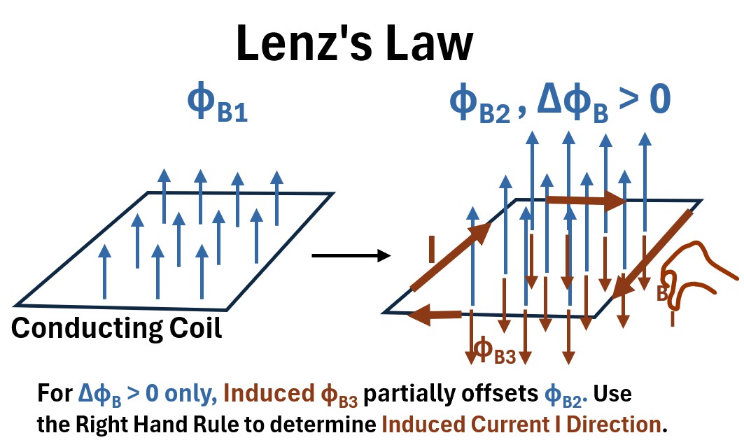
This is what happens:
(1) Change ΦB1 by amount ΔΦB which
(2) induces an Electric Field which
(3) induces a Voltage which
(4) induces Current I which
(5) induces an oppositely directed ΦB3 which
(6) partially offsets ΦB2 .
(7) Based on ΦB3 ‘s direction, use the Right Hand Rule to determine I direction (clockwise in this example).
Lenz’s Law states that the direction of an induced current is such that it creates a magnetic field that opposes the change in magnetic flux that created it.
- This is conservation of energy in action.
- It ensures that to induce a current, you must do mechanical work against a resulting opposing force.
- If the induced current did not oppose the change, it would create a self-perpetuating loop of increasing current and energy from nothing.
Lenz’s law simply states that nature abhors a change in magnetic flux.
- The induced current will always produce a magnetic field that opposes the change that caused it.
- This opposition is why the induced EMF in Faraday’s law has a negative sign
References
This section is mostly based on this great video by Sal Khan.
Motional EMF: Moving Conducting Coil and Stationary Magnetic Field
Consider a conducting coil (e.g. a circular coil) moving away from a stationary magnetic field (e.g. a magnet).
Picture: Conducting Coil Moving Away from a Magnet
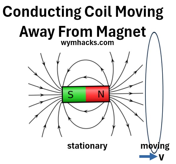
In this scenario, the coil is moved through a uniform, but spatially varying, magnetic field produced by a stationary magnet (or vice-versa), such that the flux through the coil changes.
So let’s start with our EMF equation:
EMF=∮(E̅ + v̅ x B̅)⋅dL̄
- The motion of the coil causes the term to be non-zero only along the coil’s path through the field.
- The field that arises in a moving conductor is electrostatic (conservative), meaning the net work it does on a charge moving around any closed loop is zero.
- Therefore, the E’s contribution to the net () is zero, and the entire is due to the magnetic force.
dL̄ ;
The moving charge carriers () within the coil experience a magnetic force due to their velocity () and the external magnetic field ().
- This magnetic force per unit charge is v̅ x B̅.
- This force pushes the charges along the wire, driving the current.
- This is called Motional EMF.
- The work is done by the magnetic component of the Lorentz force per unit charge, v̅ x B̅, as it moves charges around the loop.
- Note that the magnetic force does no net work on the charge over time because it is always perpendicular to the charge’s instantaneous velocity (),
- but it does work along the path of the wire to separate charges and establish the EMF.
Motional EMF: Expandable Coil in a Constant Magnetic Field
In the previous section we established a general expression for the EMF for a moving coil in a stationary magnetic field:
Motional EMF = ∮(v̅ x B̅)⋅dL̄
We can simplify this expression (i.e. get rid of the integral) if we assume we now have a conducting coil that is expandable via a moving rod that is connected to it.
It is placed (perpendicularly) into a fixed magnetic field Bo.
Picture: Movable Conducting Coil in a Fixed Magnetic Field
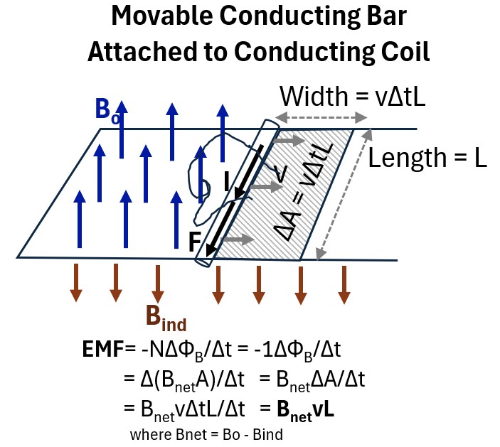
If we move the rod to the right
- for a duration of time Δt
- at a velocity v ,
- it will traverse an area ΔA equal to the product of the length of the bar (L) and the distance traversed (ΔA = vΔtL).
We are dealing with finite distances here so let’s use the average form of Faraday’s Law:
Δt
We also have an expression for magnetic flux:
ΦB = Magnetic Flux = (B)(Ap) =BAcos(θ) = B̄•Ā ; for Uniform B and Flat Surface where
Substitute for ΦB in the EMF expression to get:
Δt = Δt
because
- cos(θ) = cos(0) = 1 and
- B is constant and
- N = 1 (just one coil)
Substitute for ΔA (with vΔtL)
Δt = Δt =
So
Notice that the current that is generated (I) by the moving rod will have a clockwise direction because:
- Lenz’s Law tells us that a counter acting magnetic field will be induced .
- Use the right hand rule on (fingers pointing down) to determine that the current will go in a clockwise direction.
- In the Feynman Lectures (ch.17),for a similar example, is considered to be negligible for a weak current I.
- For completeness we can assume this is a value and we’ll just call it B.
So, in summary, looking at the drawing above, if we move the rod to the right at a velocity v,
- A motional EMF is produced (work or energy per unit charge) = BvL = (Force*Distance)/Charge
- Where B is a composite of the original magnetic field and any induced magnetic field (which is often assumed to be negligible in text book examples).
- So, a Force F is exerted on the electrons in the rod and pushes or moves the electrons (creating current I).
See this great video by Sal Khan: Emf induced in rod traveling through magnetic field
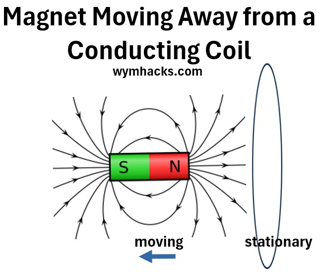
Ok, what about the scenario of a moving magnetic field and a stationary conducting coil?
Transformer EMF: Moving Magnetic Field and a Stationary Conducting Coil
In the last section we moved a coil over a stationary magnetic field and found that it is the v̅ x B̅ component of the Lorentz force that creates the EMF that causes the current to flow.
We want to imagine now that we are subjecting a stationary conducting coil to an changing magnetic field.
Picture: Moving Magnetic Field and Stationary Conducting Coil
Let’s flip the picture so we have a plan view of the coil (looking down on it from above).
This is the view you see below where
- the solid black circle is the conducting coil and
- X represents the magnetic field going into the page (symbolized as the fletching, the back end, of an arrow).
Picture: Planar View: Changing Magnetic Filed with Fixed Conducting Coil
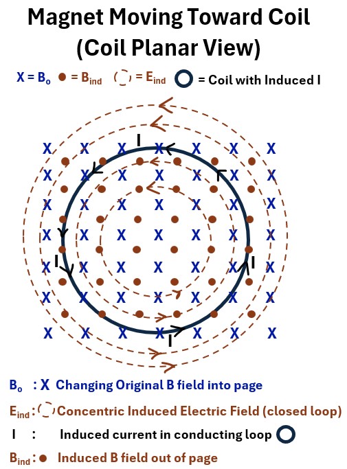
As , the original or external magnetic field, changes, a current I will begin to “flow” in the coil.
What is the responsible force that makes this happen? Let’s start with our EMF general equation:
EMF=∮(E̅ + v̅ x B̅)⋅dL̄ ; EMF Expression Using the Lorentz Force Components
There are no moving electrons to begin with in this example, so the v̅ x B̅ term is zero!
EMF= ∮Ē•dL̄ ; Transformer
So it’s an Electric field E that forces the electrons around the coil.
- But, very importantly, this E field is NOT an electrostatic field (which is a conservative field)
- E is a very unique , looping, non-conservative Electric field that is able to push the electrons around as current.
More on this E field later , but now lets go through the sequence of events that occur after this E field is created (use the picture above as you read).
- A non conservative , looping, electric field is induced.
- forms concentric closed loop circles that move counterclockwise.
- induces a magnetic field B
- We know B will be opposite according to Lenz’s Law.
- This is represented as the brown dots in the drawing above indicating the induced B field is coming out of the page.
- We can then use the right hand rule (Right hand thumb towards I and curled fingers towards B) to determine the direction of I which will be counter-clockwise.
Let’s come back to the .
is not the same as the electrostatic E field,
So, in a changing magnetic field and a stationary conducting coil, an induced electric field is created and applies the force to move the current.
But is distinctly different than the electrostatic field .
- makes loops (like B fields); has no explicit charge source; not static and always changing
- is created by stationary static charges ; i.e. it starts and stops on a charge and is static
field lines extend radially outward or inward. These fields are conservative, which means the work done by the field on a charged particle moving in a closed loop is always zero.
- So we can say the closed loop line integral on the circuit (i.e. work done) is zero i.e. W/q = ∮Ē•dL̄ = 0
- This is because the force exerted by the field is independent of the path taken and
- only depends on the starting and ending points.
- This property allows us to define an electric potential, where the work done is simply the change in potential energy between two points.
, generated by a changing magnetic field, are non-conservative.
- The work done by on a charged particle moving in a closed loop is not zero.
- There will therefore be no well defined electric potential.
The EMF term, then, is W/q = ∮Ē•dL̄
So we can write Faraday’s Law as follows:
∮Ē•dL̄ = −Nd/dt ; Transformer EMF ; Faraday’s Law of Electromagnetic Induction (line integral form relating E to B)
This equation describes the phenomenon known as Transformer EMF (or non-motional ), where the electric field is induced by a time-varying magnetic field.
- Name: It has different names
- The Maxwell-Faraday Equation (Integral Form) – One of the four Maxwell Equations.
- Faraday’s Law of Induction – Most common and general name
- Physical Meaning: The line integral of the induced electric field (E) around a stationary closed loop is equal to the negative rate of change of the magnetic flux () through the surface bounded by that loop.
- Requirement: The loop of integration (dL̄) must be stationary (fixed in space).
Eis the electric field vector. It is an induced non conservative field (its not an electrostatic field).
- dL̄ is the infinitesimal vector of a path element along a closed loop.
- The direction of this vector is tangent to the path.
- ∮ is a closed line integral. It means you are summing up the dot product of Ē and dL̄ along an entire closed loop.
- The result of this integral is the electromotive force (EMF), which is the work done per unit charge in moving a charge around the closed loop.
- For induced electric fields, this value is non-zero, indicating that the field is non-conservative.
N: # of coils
- is the magnetic flux, which is a measure of the total number of magnetic field lines passing through a given surface
- d/dt = Is the rate of change of magnetic flux with time
- −: The negative sign represents Lenz’s Law.
- It indicates that the direction of the induced electric field (and thus the induced current) will be such that it creates a magnetic field that opposes the change in the original magnetic flux.
- This is a fundamental statement of energy conservation in electromagnetism.
We also know that
ΦB = ∫sB̄•dĀ so let’s substitute this into the expression above to get
∮Ē•dL̄ = −Nd/dt = -Nd/dt∫sB̄•dĀ ; Transformer EMF ; Faraday’s Law of Electromagnetic Induction (line integral form relating E to B)
The Differential Form (The Maxwell-Faraday Equation)
This is the most fundamental and generalized form, fitting in as the final piece.
It extends the concept from a physical loop to any point in space, showing that a time-varying magnetic field (B) creates a circulating electric field (E) at a fundamental level, even in a vacuum.
It is one of the four Maxwell’s Equations and is mathematically derived from the integral form using the Divergence Theorem and Stokes’s Theorem.
- See my article, Maxwell Equations: From Integral to Differential Forms, for the derivation.
∇×Ē=-∂B̄/∂t ; Faraday Equation (Differential Form)
This equation shows how fields themselves interact dynamically.