Electricity (8/11) – Maxwell’s Equations

Maxwell’s Equations 

Electric and Magnetic Fields are inseparable and one is the origin of the other.

Maxwell’s four equations are a set of fundamental principles that describe the behavior of electric and magnetic fields and their relationship with electric charges and currents.

They are described by four fundamental equations.

Before you look at the equations, you probably need a little review of the key mathematical operators that are used.

In this section I’ll present the equations with a little bit of explanation.

If you really want to get a more complete understanding, then read my dedicated posts:

Maxwell Equations; From Integral to Differential Forms

From Maxwell’s Equations to The Wave Equation

Ampère Maxwell Equation

Note that E, B, J, dA, dL are all vectors and have magnitude and direction. 

These can also be written with bars on top of the letters

i.e. E̅ , B̅,  J̅,  dA̅,  dL̅ 

Gradient, Diversion, and Curl Operators

In order to understand the Maxwell equations, you need to understand the concept of vectors, fields and the math of gradients, divergence, and curls.

So read my posts:

• Vector Math
• Field Operators: Gradient, Divergence, and Curl

Some of the key concepts are:

Vector Field

A vector field is a collection of vectors (quantities that have both magnitude and direction), one at every point in space.

Think of it like a wind weather map.

• For a select areas of a city, or state, or region, etc. arrows are shown.
• Each arrow’s length shows the wind’s speed,
• and its direction shows the way the wind is blowing.

Divergence Operator ∇⋅ 

Divergence is a measure of how much a vector field “spreads out” from a point (think of water spraying out of a sprinkler or water flowing into a drain).

Curl Operator ∇×

The curl operator measures how much a vector field rotates around a point.

Forms or Versions of the Maxwell Equations

Each of the four laws can be expressed in either the integral form or the differential form.

While they describe the exact same physical phenomena, they offer different perspectives:

• The Integral Form looks at the “big picture,” describing how fields behave over entire volumes or around large loops.
• The Differential Form zooms in to a single point in space, using calculus to show how fields vary and interact locally.

Together, these dual representations provide a complete toolkit for solving electromagnetic problems, whether you’re analyzing a massive planetary magnetic field or a microscopic circuit.

In the following sections we’ll review both forms of each of the Maxwell Equations.

Maxwell Equations Integral and Differential Forms

1. Gauss’s Law (for Electric Fields or Electrostatics)

• Integral Form:        ∮_SE̅⋅dA̅ = Q_enc/ε₀    
• Differential Form:  ∇⋅E̅ = ρ/ε₀ = 4πkρ
• Meaning:
  • Electric charges produce an electric field.
  • Electric fields E̅ act in a divergent way (∇⋅E̅) ,
  • meaning they are flowing outward or inward.
  • An electric charge (expressed on the right hand side of the equation) acts as a source for the electric field E̅.
  • Any time you have a charge, that charge will create an Electric Field (which exerts a force)

2. Gauss’s Law for Magnetic Fields

• Integral Form:        ∮_SB̅⋅dA̅ = 0
• Differential Form:  ∇⋅B̅ = 0
• Meaning:
  • You’ll never see divergent behavior from magnetic fields

  • Standalone magnetic charges cannot exist.

  • There are no magnetic monopoles; magnetic field lines are continuous loops.
  • There is no such thing as a magnetic charge (there are no magnetic mono-poles).
  • You can’t have a north pole without a south pole.
  • Magnetic fields do not originate from charges or any other point sources (or syncs).
  • Magnetic field lines are continuous loops.

3. Faraday’s Law of Induction

• Integral Form:        ∮_CE̅⋅dL̅ = V =  −dΦ_B/dt    
• Differential Form:  ∇×E̅ = −∂B̅/∂t
• Meaning:
  • A changing (with time) magnetic field (∂B̅/∂t) induces a curling (rotating) electric field (∇xE)
  • A changing magnetic field creates an electric field, which is the principle behind electric generators.
  • If a closed conductive path is available, this electric field will cause a current to flow in that path.
  • A changing magnetic field induces an electromotive force ∮_CE̅⋅dL̅
  • i.e pushing a magnet back and forth in a coil of wire causes the magnetic field B to change,
  • which disturbs the electric field E and sets electrons in motion.
  • This induction creates electric current.

These amazing equations explain our modern power creation and distribution technologies. 

See my posts on transformers and electric generators:

• Alternating Current (AC) Generation
• Transformers

 4. Ampère-Maxwell Law

• Integral Form:  ∮_CB̅⋅dL̅ =μ₀(I_enc+ε₀dΦ_E/dt)
• Differential Form:  ∇×B̅=μ₀(J̅+ε₀∂E̅/∂t)
• Meaning:
  • Magnetic fields are generated by moving charges (current) and changing electric fields.
  • It is the foundation for understanding how electromagnetic waves (like light) propagate
  • It relates the magnetic field around a closed loop to the total current passing through the surface enclosed by that loop.
  • It shows that the “curl” (rotation) of the magnetic field at a point is caused by
    • the local Current Density J̅ and
    • the local rate of change of the electric field: the term ε0∂Ē/∂t is called the Displacement Current.
    • That is, an electric current or a change in the electric field leads to a disturbance of the magnetic field.
• Both Faraday’s Law and the Ampere Maxwell say that change in the magnetic field B̅ disturbs the electric field E̅ and vice versa.
  • This alternation between E̅ and B̅ allows electromagnetic energy to propagate in the form of waves,
  • which travel at the speed of virtual photons i.e. electromagnetic waves.
  • They include microwaves, x-rays, infrared or even light.

Maxwell Equation Variables and Terms

Note that E, B, J, dA, dL are all vectors and have magnitude and direction. 

Sometimes this is indicated by bolding the letters and/or putting lines on top of them.

i.e. E̅ , B̅,  J̅,  dA̅,  dL̅   

• E̅  / Electric (Vector) Field / Volts per meter (V/m)
• B̅  / Magnetic Flux Density (Magnetic Field) / Tesla (T)
• ρ  /  Total Charge Density / Charge per Volume / Coulombs per cubic meter (C/m³)
• J̅  / Current Density (I/A) / Amperes per square meter (A/m²)
  • J̅ is the flow of actual electric charges (like electrons in a wire) per unit area
• Qenc / Enclosed Electric Charge/Coulomb (C)
• Ienc / Enclosed Electric Current ; The net “traditional” current piercing the surface. / Ampere (A)
  • The actual flow of electric charges (electrons) passing through the surface area bounded by your loop
• Φ_E  / Electric Flux / V⋅m
• Φ_B / Magnetic Flux/Weber (Wb)

• ∮_SE̅⋅dA̅/ Total Electric Flux

  • This represents the net sum of the electric field passing through a closed 3D boundary.
  • It “counts” the electric field lines exiting or entering a “bubble.” If more lines leave than enter, the flux is positive.
  • It is the macroscopic way to measure the presence of charge inside a volume without looking inside
• ∇⋅E̅/ Divergence of E̅
  • This describes the field’s behavior at an infinitesimal point.
  • It measures the “outgoingness” of the field. A positive divergence means the point acts as a source (like a nozzle spraying water); a negative divergence means the point is a sink (like a drain).

• ∮_SB̅⋅dA̅ / The Total Magnetic Flux

  • This sums up the magnetic field lines passing through a closed 3D surface (a “bubble”).
• ∇⋅B̅/ The Divergence of B̅
  • This measures the “spreading out” or “concentration” of the magnetic field at a single, infinitesimal point in space.

• ∮_CE̅⋅dL̅ / Electromotive Force or Circulation

  • The “sum” of the electric field along a closed loop (C).
• −dΦ_B/dt / Rate of Change of Magnetic Flux
  • The time derivative (rate of change) of the total magnetic flux (Φ_B) passing through the surface area bounded by the loop

• ∇×E̅ / Curl of the Electric Field

  • It describes a vortex or “swirl” in the electric field
• −∂B̅/∂t  /Time-Varying Magnetic Field
  • The partial derivative of the magnetic field vector with respect to time at a specific location

• ∮_CB̅⋅dL /Magnetic Circulation

  • This measures the total “circulation” of the magnetic field around the loop.
• ε₀dΦ_E/dt  / Displacement Current
  • This represents a changing electric flux
• ∇×B̅ / The Curl of the Magnetic Field
  • measures the rotation or “swirl” of the magnetic field B
  • ∇xB̅ = μ0J is the original Ampere’s Law
• μ₀ε₀∂E̅/∂t / Displacement Current /  Amperes per square meter (A/m²)
  • A changing electric field acts just like a physical current.
  • The rate at which the electric field is changing over time at that specific point
  • Displacement current isn’t actually “current” (moving charges); it’s a changing electric field that acts like a current by producing a magnetic field.
  • Added by Maxwell to Ampere’s Law.
  • It’s Maxwell’s “mathematical glue” that ensures magnetic fields still exist in gaps—like between capacitor plates—where physical electrons aren’t flowing

Maxwell Equation Constants

• ε₀ = electric permittivity of free space (a constant) /  8.854×10−12 F/m
• μ₀ = magnetic permeability of free space (a constant) / 4π×10−7 H/m
• k = Coulomb’s Constant = 1/(4π ε₀)
• c   = speed of light in a vacuum = 1/sqrt(μ₀ε₀) =  299,792,458 m/s
• π = pi = 3.1415..

Maxwell’s Equations Operators

• ∇
  • Del (Nabla)
  • Vector differential operator
  • Represents the rate of change in 3D space.
• ∇⋅
  • Divergence Operator (Nabla dot)
  • “Flux per unit volume”
  • Measures if a field is “spreading out” from a point (source) or “shrinking” into it (sink).
• ∇×
  • Curl
  • “Rotation”
  • Measures the tendency of a field to circulate or “spin” around a point.
• ∂/∂t
  • Partial Time Derivative
  • Temporal change
  • Measures how the field changes at a fixed point as time passes.
• ∮_S
  • Surface Integral
  • Total flux through a surface
  • Sums the field components passing perpendicularly through a closed surface.
• ∮_C
  • Line Integral
  • Circulation around a path
  • Sums the field components tangent to a closed loop.
• dA̅
  • Differential Area
  • Vector Surface element
  • A vector normal (perpendicular) to the surface.
• dL̅
  • Differential Path Vector
  • Path element
  • A tiny vector tangent to the integration loop.

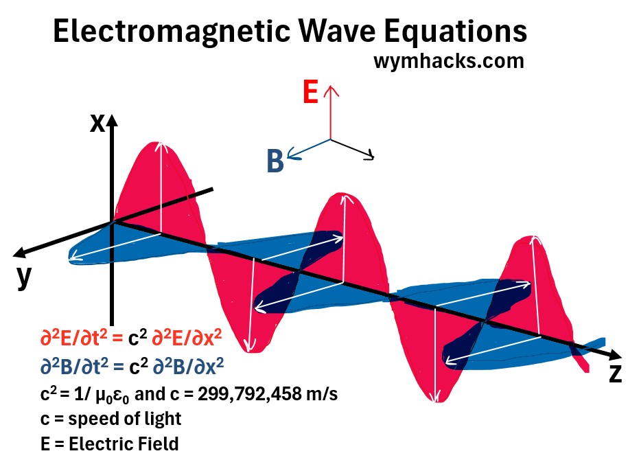
Wave Equations

Clearly, Maxwell did not discover all these equations.

• The first two equations  are based on the work of Carl Friedrich Gauss,
• The third equation is based on the work of  Michael Faraday,
• The μ₀J̅ part of the 4th equation is based on the work of  André-Marie Ampère.

But, Maxwell brilliantly synthesized them by

• adding the displacement current term, μ₀ε₀∂E/∂t to the fourth equation
• and deriving wave equation forms for the electric and magnetic field terms.

So, Maxwell’s greatest achievement was manipulating his equations to

• predict electromagnetic waves, and
• show that Light waves were a form of electromagnetic wave.

∂2E̅/∂t2 = c2 ∂2E̅/∂x2  =  Wave Equation for the Electric Field

∂2B̅/∂t2 = c2 ∂2B̅/∂x2  =  Wave Equation for the Magnetic Field

c² = 1/ μ₀ε₀ and c = 299,792,458 m/s

His profound conclusion that light itself was an electromagnetic wave was later proven true and laid the groundwork for modern physics and technology

Graph: Electromagnetic Wave Graph and Equations

See my post From Maxwell’s Equations to The Wave Equation to

• get more details on Maxwell’s Equations and
• see how the wave equations can be derived for magnetic and electric fields B̅ and E̅.

Great Educational Resources

• Faraday, Maxwell, and the Electromagnetic Field – By Nancy Forbes and Basil Mahon – 2019 Prometheus Books
• You don’t understand Maxwell’s equations – Ali the Dazzling
• Maxwell’s Equations Visualized (Divergence & Curl) – Science Asylum
• The Wave Equation simplified – Ali the Dazzling

Return to Menu