Menu (linked Index)
From Maxwell’s Equations to The Wave Equation
Last Update: August 20, 2025
Introduction
James Clerk Maxwell (1831–1879) was a Scottish physicist known for his groundbreaking work in electromagnetism.
In the 1860s, he synthesized (and contributed to) the work of previous scientists like Faraday and Ampère into (ultimately) a set of four partial differential equations.
These equations (today called Maxwell’s equations) are a set of four fundamental equations that describe how Electric and Magnetic fields behave and how they relate to each other.
If you want to learn more about Maxwell
- and Michael Faraday who inspired him, and
- Oliver Heaviside who invented the math to make his theories more understandable,
- and the other great scientists who contributed to or proved them,
then read the book “Faraday, Maxwell, and the Electromagnetic Field” by Forbes and Mahon.
Also, use the appendices 1 (educational resources), 2 (equation history summary), and 3 (detailed equation history) to learn more.
Maxwell’s Equations establish the fundamental rules of electromagnetism i.e.
- Electric fields originate from charges.
- Magnetic fields do not originate from charges or any other point sources (or syncs).
- Magnetic field lines are continuous loops.
- A changing magnetic field creates an electric field.
- A changing electric field or a flow of current creates a magnetic field.
Together, these four equations predict the existence of electromagnetic waves, which travel at the speed of light.
They unified the previously separate fields of electricity, magnetism, and optics into a single, elegant theory.
Before we delve into the equations, you need a little tutorial on the Grad, Div and Curl operators.
Gradient, Diversion, and Curl Operators
For a deeper understanding of vector fields and field operators (gradient, diversion, curl), please read my post Field Operators: Gradient, Diversion, and Curl.
My post will give you a much better visual feel for what is going on with vectors and what the vector operators do.
The Del Operator
The del operator, denoted by the symbol ∇, is a vector differential operator.
You can think of it as a vector whose components are partial derivative operators.
In three-dimensional Cartesian coordinates (x,y,z), it’s defined as:
The Del Operator = Nabla = ∇ = (∂/∂x)î + (∂/∂y)ĵ + (∂/∂z)k̂
- where î, ĵ, k̂ are the unit vectors in the x, y, and z directions, respectively.
- and nabla is the ancient Greek word for a certain type of harp (shape looks like a harp).
The Del Operator or Nabla is used in the Gradient Operator, the Divergence Operator and the Curl Operator.
The Gradient Operator
If f(x,y,z) is a scalar field, its gradient is a vector field:
Gradient of f = grad f = ∇f = (∂f/∂x)î + (∂f/∂y)ĵ + (∂f/∂z)k̂
- The gradient vector points in the direction of the steepest increase of the scalar field.
- Imagine a topographical map where the scalar field is the elevation.
- The gradient at any point would be a vector pointing straight up the hill, indicating the path of fastest ascent.
- The magnitude (or length) of the gradient vector represents the rate of change in that steepest direction.
The Divergence Operator
If F(x,y,z) = Fxî + Fy ĵ + Fzk̂ is a vector field,
its divergence is a scalar field given by:
Divergence of F = div F = ∇⋅F =∂Fx/∂x + ∂Fy/∂y + ∂Fz/∂z
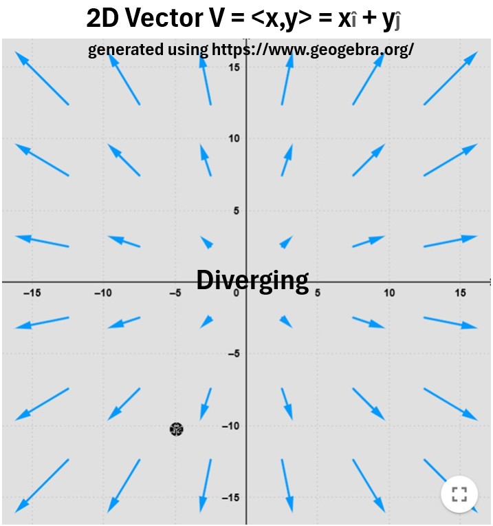
Divergence measures how much stuff is sourcing out or in (syncing)
- Think of a water faucet splashing on a surface; positively divergent… or
- water flowing downward into a drain…negatively divergent.
Check out this video for a nice visual explanation of the divergence: Divergence intuition, part 1
Picture: Example of a 2 D Diverging Vector Field
The Curl Operator
For the same vector field F(x,y,z), the curl is a vector field given by:
Curl of F = curl F = ∇×F
= (∂Fz/∂y − ∂Fy/∂z )î
– (∂Fz/∂x – ∂Fx/∂z)ĵ
+ (∂Fy/∂x – ∂Fx/∂y)k̂
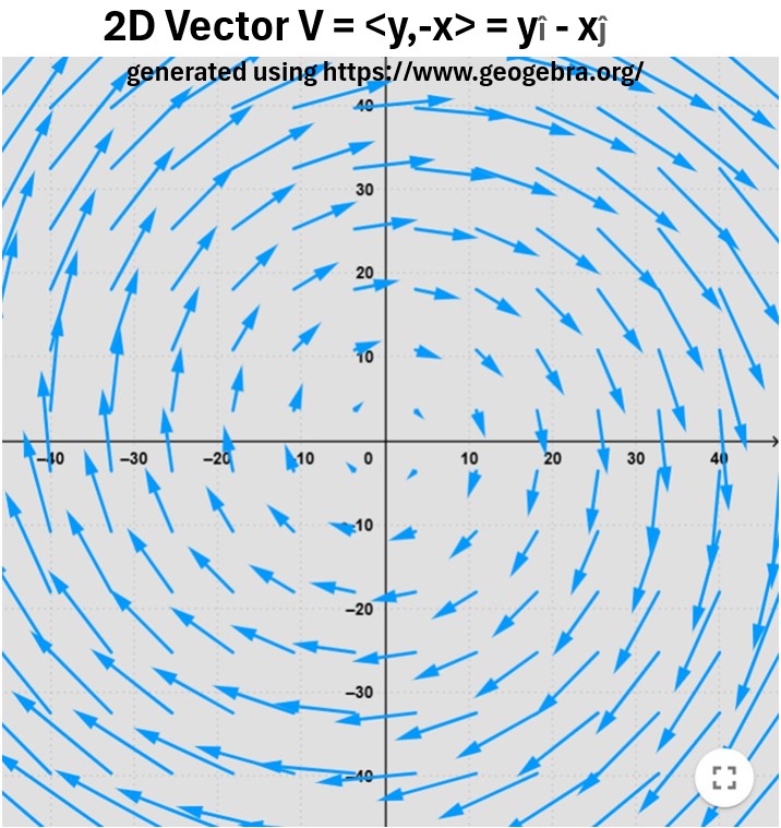
The curl indicates rotation.
It tells you how much a vector field “curls” or “swirls” around a point.
- Imagine a tiny paddlewheel placed in a flowing fluid.
- If the paddlewheel starts to spin, the fluid has a non-zero curl.
- The direction of the curl vector points along the axis of rotation of the paddlewheel, and
- its magnitude represents the speed of the rotation.
Check out this video for a nice visual explanation of the curl: 2d curl intuition
Picture: Example 2D Curling Vector Field
Maxwell’s Equations (ME)
Watch these two great videos providing a high level description of what these equations mean.
- You don’t understand Maxwell’s equations – Ali the Dazzling
- Maxwell’s Equations Visualized (Divergence & Curl) – Science Asylum
and don’t forget Appendix 1 for more great references.
Oliver Heaviside
Maxwell’s original work on electricity and magnetism was expressed in a complex set of over 20 equations using quaternions, a mathematical language that was not widely understood at the time.
Oliver Heaviside, a self-taught English physicist and engineer, applied a new mathematical system, vector calculus, to Maxwell’s theory.
He simplified the original equations by condensing them into the four concise vector equations that are now taught in physics and engineering.
So, we’ll use these 4 “Maxwell-Heaviside” forms of the equations below.
Refer to Appendices 2 and 3 for more on the history of the Maxwell Equations.
Maxwell Equations Meanings
Ok, lets jump into what the equations look like (ME1, ME2, ME3, ME4) and what they mean.
ME1: ∇⋅E = ρ/ε0 = 4πkρ
This is Gauss’s Law for an electric field E.
Gauss’s Law for the Electric Field states that:
- a charge Q (where ρ = charge/volume) creates an electric field E.
- electric fields E act in a divergent way (∇⋅E) , meaning they are flowing outward or inward.
- An electric charge acts as a source or sync for the electric field E.
Variable Descriptions
- ∇⋅ = Divergence Operator where ∇ = nabla or del.
- E = Electric Vector Field
- ρ = charge density = charge/volume = Q/V
- ε0 = electric permittivity of free space
- It is a fundamental physical constant that represents the ability of a vacuum to permit electric field lines.
- ε0 = 8.854×10⁻¹² Farads per meter (F/m)
- k = Coulomb’s Constant = electrostatic constant = 1/(4π ε0) ≈8.99×10⁹ N⋅m2/C2
- μ0 = magnetic permeability of free space = magnetic constant = 4π×10-7 H/m (Henrys per meter).
- It is a fundamental physical constant that describes how a vacuum responds to a magnetic field.
- c = 1/sqrt(μ0ε0) = speed of light = 299,792,458 m/s
- π = pi = 3.1415..
ME2: ∇⋅B = 0
This is Gauss’s Law for a magnetic field.
It states that standalone magnetic charges cannot exist.
- There is no such thing as a magnetic charge (there are not magnetic mono-poles).
- You can’t have a north pole without a south pole.
- Magnetic fields do not originate from charges or any other point sources (or syncs).
- Magnetic field lines are continuous loops.
ME3: ∇xE = -∂B/∂t
This is Faraday’s Law (of Induction) or the law of Electrical (or Electromagnetic) Induction.
It states that
- a changing (with time) magnetic field (∂B/∂t) induces a curling (rotating) electric field (∇xE)
- and, if a closed conductive path is available, this electric field will cause a current to flow in that path.
Another statement of it is
- a disturbance in the magnetic field B affects the electric field E.
- i.e pushing a magnet back and forth in a coil of wire causes the magnetic field B to change,
- which disturbs the electric field E and sets electrons in motion.
- This induction creates electric current.
ME4: ∇xB = μ0J + μ0ε0∂E/∂t
This is sometimes referred to as the Ampere-Maxwell Law (or Ampere’s Law with Maxwell Addition).
- ∇xB = the curl (rotation indicator) of the magnetic field B
- J = current density = I/A = Current/Area
- ε0 = electric permittivity of free space
- μ0 = magnetic permeability of free space
- ∇xB = μ0J is the original Ampere’s Law
- μ0ε0∂E/∂t is called the displacement current and was added by Maxwell.
ME4 says that: An electric current or a change in the electric field leads to a disturbance of the magnetic field.
- A change in the magnetic field B disturbs the electric field E and vice versa.
- This alternation between E and B allows electromagnetic energy to propagate in the form of waves,
- which travel at the speed of virtual photons i.e. electromagnetic waves.
- They include microwaves, x-rays, infrared or even light.
Clearly, Maxwell did not discover all these equations.
- ME1 and ME2 are based on the work of Carl Friedrich Gauss,
- ME3 is based on the work of Michael Faraday,
- The μ0J part of ME4 is based on the work of André-Marie Ampère.
But, he brilliantly synthesized them by
- adding the displacement current term, μ0ε0∂E/∂t to ME4
- and deriving wave equation forms for the electric and magnetic field terms.
Let’s learn a little about the wave equation before I show how we can transform the Maxwell equations into wave equation form.
The Wave Equation
The mathematical form of the wave equation was known in Maxwell’s time, and this knowledge was crucial to his discovery.
Physicists and mathematicians of the 18th century, such as Jean-Baptiste d’Alembert (circa 1746) and Leonhard Euler (circa 1756), had already developed the
- one-dimensional and
- three-dimensional wave equations
- to describe phenomena like sound waves and vibrating strings.
The general form of the wave equation for a scalar quantity ψ in a medium with propagation speed v is:
(∂2ψ/∂x2 + ∂2ψ/∂y2 + ∂2ψ/∂z2) = (1/v2)∂2ψ/∂t2
or re-arranged,
∂2ψ/∂t2 = v2(∂2ψ/∂x2 + ∂2ψ/∂y2 + ∂2ψ/∂z2)
Example of a Wave Equation in One Dimension
Lets translate this equation into a simple real world example where
- we are dropping a pebble into the calm surface of a pond.
- we are only looking at a one dimensional view of a pond surface (i.e. on a 1D x axis).
- u is the “wave function” which is really a vertical displacement function.
∂2u/∂t2 = v2(∂2u/∂x2) : 1 D Wave Equation
In this one-dimensional wave equation for a pebble dropped in a pond, u and x represent the following:
- u represents the disturbance,
- which is the vertical displacement of the water’s surface from its resting, flat position.
- x represents the position along the horizontal direction of wave travel, which is the path the wave is propagating along.
- It is a distance from the point where the pebble was dropped.
So, at any point in time t,
- the value of u changes as you move along the x-axis.
- the wave equation describes how this disturbance propagates over time and space,
- relating the acceleration of the water’s vertical displacement to its curvature.
∂2u/t2 is an acceleration term since
- the derivative of displacement is velocity
- and the derivative of the velocity (or second derivative of the displacement) is the acceleration
The second spatial derivative, ∂2u/∂x2
- is the mathematical representation of this curvature.
- It tells you how the slope of the disturbance is changing.
Ok, we now have a decent feel for what a wave equation is.
When Maxwell manipulated his electromagnetism equations, he derived equations for both the electric field E and the magnetic field B that had this exact wave form.
Deriving the Electromagnetic Wave Equations From Maxwell’s Equations
The following derivation uses the modern “Heaviside” versions of the Maxwell equations, so Maxwell himself did not use the exact methodology we’ll follow.
But he, of course, arrived at the same wave equation solutions.
Let’s do it.
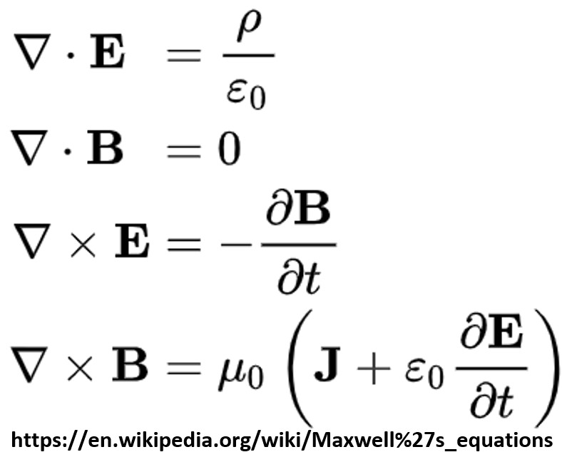
Starting with the Maxwell Equations,
ME1: ∇⋅E = ρ/ε0 = 4πkρ (Gauss’s Law of E)
ME2: ∇⋅B = 0 (Gauss’s Law of B)
ME3: ∇xE = -∂B/∂t (Faraday’s Law)
ME4: ∇xB = μ0J + μ0ε0∂E/∂t (Ampere-Maxwell law)
Assume vacuum conditions hold; i.e. free space i.e. no charges.
So, ρ and J become zero and ME1 through 4 become:
(1) ∇⋅E = 0
(2) ∇⋅B = 0
(3) ∇xE = -∂B/∂t
(4) ∇xB = μ0ε0∂E/∂t
The only other thing we need is the following vector identity where it is always true that,
(5) ∇x(∇xF) = ∇(∇⋅F) – ∇2F
In this analysis F = E or B.
Since ∇⋅E = 0 and ∇⋅B = 0, we can rewrite (5) as
(6a) ∇x(∇xE) = – ∇2E
(6b) ∇x(∇xB) = – ∇2B
Derivation of the Electric Field Wave Equation
Take the curl of both sides of equation (3)
(7) ∇x(∇xE) = ∇x(-∂B/∂t)
Substitute (6a) into (7)
(8) –∇2E = ∇x(-∂B/∂t)
The (-) signs cancel out and we can re-organize the right hand side of (8) to get
(9) ∇2E =∂/∂t(∇xB)
Substitute for ∇xB using equation (4), so equation (9) becomes
(10) ∇2E =∂/∂t(μ0ε0∂E/∂t)
Manipulate (10)
- ∇2E is the Laplacian which is ∂2E/∂x2 in 1 D space.
- Express right hand side as a second order derivative.
- Swap the left and right hand sides.
to get:
(11) ∂2E/∂t2 =(1/μ0ε0)∂2E/∂x2
which looks a lot like a wave equation of the form
∂2u/∂t2 = v2(∂2u/∂x2)
Imagine how amazed and excited Maxwell must have been when he discovered that (1/μ0ε0) = v2 .
When he plugged in the values for the constants μ0ε0 and computed v , he got
- 310,740 km/s which was very close
- to 314,850 km/s; the speed of light computed by Armand Hippolyte and Louis Fizeau.
Maxwell’s value is only different from the actual speed of light ( 299,792,458 meters per second) do to inaccuracy of the constants used.
So the v term in equation (11) is indeed the speed of light c
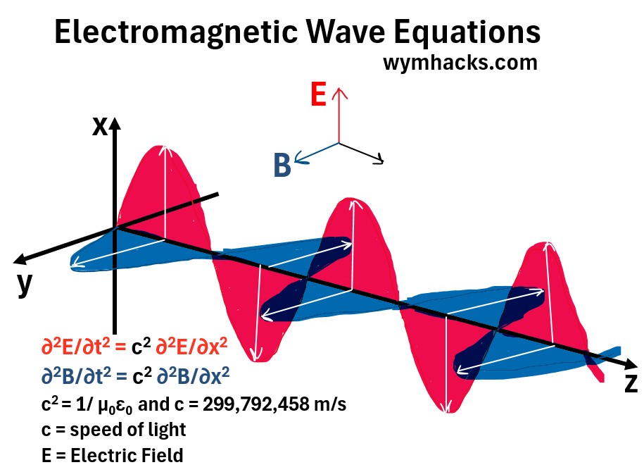
(12) ∂2E/∂t2 = c2 ∂2E/∂x2 = Wave Equation for the Electric Field
(13) c2 = 1/ μ0ε0 and c = 299,792,458 m/s
Derivation of the Magnetic Field Wave Equation
We follow the same steps to derive the magnetic field wave equation.
Take the curl of both sides of equation (4)
(14) ∇x(∇xB) = ∇x(μ0ε0∂E/∂t)
Substitute (6b) into (14)
(15) –∇2B = ∇x(μ0ε0∂E/∂t)
Re-organize the right hand side of (15) to get
(16) –∇2B =μ0ε0∂/∂t(∇xE)
Substitute for ∇xE using equation (3), so equation (16) becomes
(17) –∇2B =μ0ε0∂/∂t(-∂B/∂t)
Manipulate (17)
- Minus signs cancel.
- ∇2B is the Laplacian which is ∂2B/∂x2 in 1 D space.
- Express right hand side as a 2nd order derivative.
- Swap the left and right hand sides.
to get:
(18) ∂2B/∂t2 =(1/μ0ε0)∂2B/∂x2
so
(19) ∂2B/∂t2 = c2 ∂2B/∂x2 = Wave Equation for the Magnetic Field
(20) c2 = 1/ μ0ε0 and c = 299,792,458 m/s
Graph: Electromagnetic Wave Graph and Equations
Interpretation and Significance of the E and B Wave Equations
note: I used Google Gemini to generate the description below (based on the EM wave drawing above).
To understand the wave equations of the magnetic and electric fields, imagine a light beam traveling in the z-direction (see graph above).
- This light beam isn’t just a simple ray; it’s a dynamic disturbance with two inseparable components
- that oscillate at right angles to each other and to the direction of propagation.
The Electric Field Component
Think of the electric field as an invisible, vertical rope that’s attached to the light beam.
- As the light beam moves forward (in the z-direction), this rope whips up and down, creating a wave.
- The height of the rope’s displacement at any point represents the strength of the electric field at that location.
- This vertical oscillation is confined to the x-z plane (or another plane perpendicular to the magnetic field).
- The wave equation for the electric field describes how this vertical wave propagates through space and time.
The Magnetic Field Component
Simultaneously, imagine a second, invisible, horizontal rope attached to the same light beam.
- This rope represents the magnetic field.
- As the light beam moves forward, this second rope whips left and right, creating its own wave.
- The horizontal displacement of this rope represents the strength of the magnetic field.
- This oscillation is confined to the y-z plane (or another plane perpendicular to the electric field).
- The magnetic field’s wave equation describes the propagation of this horizontal wave.
The Interplay and The Wave Equations
The key to this analogy is that these two oscillations—the vertical electric field wave and the horizontal magnetic field wave—are not independent.
- They are inextricably linked.
- The changing electric field creates the magnetic field, and the changing magnetic field creates the electric field.
- This mutual creation and sustenance allow both waves to propagate together, perpetually “feeding” each other. .
- The wave equations for the electric and magnetic fields are mathematical descriptions of this dance.
- They show that both fields propagate at the speed of light (c) and are solutions to the same type of second-order partial differential equation.
- This means they are both sinusoidal waves that travel together, in phase and at the same speed, through a vacuum.
Watch these great videos:
Appendix 1: Information and Sources: Maxwell Equations
- Faraday, Maxwell, and the Electromagnetic Field – By Nancy Forbes and Basil Mahon – 2019 Prometheus Books
- The Engines of Our Ingenuity – Maxwell and Faraday
- The Unification of Electricity and Magnetism
- You don’t understand Maxwell’s equations – Ali the Dazzling
- Maxwell’s Equations Visualized (Divergence & Curl) – Science Asylum
Kathy Loves Physics Videos are Awesome
- James Clerk Maxwell Biography: History of Maxwell’s Equations
- Maxwell’s Equations Explained: Supplement to the History of Maxwell’s Eq.
- How Heinrich Hertz Discovered Radio to Validate Maxwell’s Equations
Parth G Videos
- Let There Be Light: Maxwell’s Equation EXPLAINED for BEGINNERS
- Excellent visual descriptions of the meaning of vector fields and their divergence and/or curl.
- Here’s What Maxwell’s Equations ACTUALLY Mean.
- Really nice but be aware that
- his description of the 4th equation (Ampere Maxwell law) contains an error.
- Error Description: The term Maxwell added, the displacement current, was the dE/dt term, not the J term (that was already in Ampere’s Law)
Deriving The Wave Equations for B and E from Maxwell’s Equations
Appendix 2 – A History of Maxwell’s Equations
Maxwell Equations Publications
On Physical Lines of Force
- Published in 1862;
- 20 Equations;
- Quaternions and Cartesian coordinates
- Introduced the concept of the displacement current and magnetic vortices; derived equations for the electromagnetic field.
- Unified electricity and magnetism for the first time; laid the groundwork for the prediction of electromagnetic waves.
A Dynamical Theory of the Electromagnetic Field
- Published in 1865 (3 years after first publications by Maxwell)
- 8 equations in component form; Quaternions and vector calculus-like notation
- Combined the 20 equations into 8 more elegant equations;
- Explicitly predicted the existence of electromagnetic waves and calculated their speed.
- This formulation is often considered the most complete and the one that first explicitly predicted light as an electromagnetic wave.
A Treatise on Electricity and Magnetism
- Published in 1873 (11 years after first publications by Maxwell)
- 4 sets of equations (20 in total); Quaternions and vector calculus-like notation
- Presented a comprehensive, detailed, and accessible treatment of the theory;
- The equations were presented in a form that was widely studied and taught.
- Became the standard textbook on the subject and popularized Maxwell’s theory among a wider scientific audience.
Heaviside’s (and Gibb’s) Reformulation
- Published in 1884 (22 years after Maxwell’s first publication)
- 4 equations (vector form) using Modern Vector Calculus (∇⋅, ∇×, etc.)
- Oliver Heaviside and Josiah Gibbs condensed Maxwell’s 20 equations into the four modern vector equations we use today, making them much more concise and elegant.
- This formulation is the one now universally taught and is fundamental to all modern physics and engineering.
Heinrich Hertz
- 1887 (22 years after their prediction by Maxwell)
- Heinrich Hertz’s experimental verification of electromagnetic waves in 1887 directly confirmed Maxwell’s predictions, paving the way for the age of wireless communication.
Appendix 3 – A Definitive History of Maxwell’s Equations: From Eight Equations to the Modern Form
The Following Report was Generated using Google Gemini.
Preamble: Setting the Stage of Electromagnetism
The 19th century was a period of extraordinary intellectual ferment, but the understanding of electricity and magnetism remained fragmented and descriptive rather than unified and theoretical.
- At the time of James Clerk Maxwell’s entry into the field, the study of electromagnetism was a collection of empirical laws based on the groundbreaking work of several key figures.
- Charles-Augustin de Coulomb’s law described the force between stationary electric charges.
- André-Marie Ampère’s law provided a framework for understanding the magnetic forces generated by electric currents.
- In a separate, yet equally profound, body of work, Michael Faraday had conducted extensive experiments demonstrating the principle of electromagnetic induction, where a changing magnetic field could induce an electric current.
- Faraday, a brilliant experimentalist, conceived of “lines of force” extending through space, a qualitative and powerful concept that captured the behavior of fields but lacked a rigorous mathematical foundation.
- The scientific community, therefore, possessed a collection of powerful but disparate rules.
- These laws were effective for calculating specific outcomes under limited conditions, but they lacked a single, cohesive theoretical framework to explain the underlying principles and their interconnectedness.
- The concept of an “electromagnetic field” was still a nascent idea, with most physicists viewing forces as actions at a distance.
- This intellectual environment presented a profound challenge: to synthesize these isolated phenomena into a single, comprehensive theory that could not only describe existing observations but also predict new ones.
- James Clerk Maxwell, a Scottish physicist and mathematician with a unique ability to bridge the gap between abstract mathematics and physical reality, was uniquely suited to this task.
The Foundational Work: From Mechanical Analogy to Theory
Early Formulations: The Twenty Equations of On Physical Lines of Force
Maxwell’s intellectual journey toward a unified theory began with a series of papers titled On Physical Lines of Force, published between 1861 and 1862.
- In this foundational work, he set out to translate Faraday’s qualitative concept of lines of force into a quantitative, mathematical theory.
- To achieve this, Maxwell employed a bold and imaginative mechanical analogy. He visualized the electromagnetic field as a complex system of “molecular vortices” representing magnetic lines of force, separated by a layer of “idle wheels” representing electric charge.
- This intricate, albeit cumbersome, mechanical model allowed him to deduce mathematical relationships between electric and magnetic phenomena.
- The culmination of this initial effort was a set of twenty component-based equations.
- These equations, which were expressed without the benefit of modern vector calculus, were highly complex and difficult to work with.
- However, they represented a significant achievement, for they marked the first time that a mathematical system had been proposed to describe the interconnected dynamics of electric and magnetic fields.
- This was a crucial first step in turning Faraday’s intuitive ideas into a rigorous physical theory.
The Birth of the Displacement Current
Within the framework of this mechanical model, Maxwell made his most profound and original contribution: the theoretical introduction of the “displacement current”.
- This term was a daring addition to Ampère’s Law, which originally only accounted for magnetic fields generated by electric currents in a wire.
- Maxwell’s analysis revealed a logical inconsistency in Ampère’s Law when applied to a charging capacitor, where the current appears to be discontinuous.
- To resolve this, he proposed that a changing electric field, even in a vacuum, could produce a magnetic field just like a conventional electric current.
- The physical significance of this theoretical construct cannot be overstated.
- It was not a change in mathematical notation or a simplification of existing ideas; it was a novel physical concept that fundamentally altered the understanding of electromagnetism.
- The introduction of the displacement current was the key that unlocked the true dynamism of the electromagnetic field.
- Without this term, Maxwell’s equations would have described a set of static relationships, unable to predict the existence of self-propagating electromagnetic waves.
- This single theoretical stroke of genius allowed for the existence of waves moving through a vacuum, thereby forging the link between electricity, magnetism, and light.
- The intellectual leap from a descriptive model of forces to a dynamic field theory, facilitated by the displacement current, is the true heart of Maxwell’s achievement.
The Landmark Publication: A Dynamical Theory of the Electromagnetic Field (1865)
The seminal paper, A Dynamical Theory of the Electromagnetic Field was read before the Royal Society on December 8, 1864, and subsequently published in the 1865 volume of the Philosophical Transactions of the Royal Society of London.
This paper represents the pinnacle of his theoretical work, where he moved away from the cumbersome mechanical analogies of his earlier papers and presented a more abstract and elegant mathematical formulation of his field theory.
The Analysis of the 1865 Formulation
The 1865 publication contained Maxwell’s refined set of eight equations, which were presented in a more compact and elegant form than his earlier twenty-equation set.
- These equations, while still complex by today’s standards, were a significant step forward, representing the core principles of his theory.
- They described the relationships between electric field strength (E), magnetic induction (B), electric displacement (D), and magnetic field intensity (H).
- This set included his groundbreaking addition of the displacement current, which was now fully integrated into the theory.
- The true power of this new formulation was its predictive capability.
- By combining his equations, Maxwell was able to derive a wave equation for the electromagnetic field.
- He calculated the velocity of these waves based on fundamental constants of electricity and magnetism, specifically the ratio of the electrostatic to the electromagnetic unit of charge.
- His calculation yielded a value of approximately 310,740 kilometers per second, which was astonishingly close to the experimental value for the speed of light, which was known at the time to be around 315,300 kilometers per second.
- This stunning agreement led Maxwell to a profound and world-changing conclusion: light is an electromagnetic wave.
- This unification of optics with electromagnetism was a monumental achievement in the history of science, providing a single, coherent theory for phenomena that had previously been considered entirely separate.
The Road to Modernity: Consolidation and Simplification
The Consolidation: The Treatise on Electricity and Magnetism (1873)
Following the success of his 1865 paper, Maxwell dedicated himself to producing a comprehensive and definitive text on the subject. The result was his two-volume magnum opus, the Treatise on Electricity and Magnetism, published in 1873.
- This work was intended to be a foundational text for the entire field of electricity and magnetism, summarizing not just his own contributions but the entirety of the existing knowledge.
- The Treatise is often mistakenly cited as the source of the modern four equations.
- However, the reality is that the equations in this work were even more numerous and complex than the 1865 set.
- They were still presented in a cumbersome form, using a mix of quaternion notation and a total of over twenty scalar equations to represent the full theory.
- While a masterpiece of theoretical physics, its complexity made it difficult for the average physicist or engineer to interpret and apply.
The Simplification: Heaviside, Gibbs, and the Birth of Vector Calculus
The transformation of Maxwell’s theory from a complex, inaccessible masterpiece into the elegant and widely used cornerstone of modern physics was not the work of a single person, but a collaborative effort.
- Following Maxwell’s death in 1879, two brilliant minds independently undertook the task of simplifying his work.
- Oliver Heaviside, an English electrical engineer, and Josiah Willard Gibbs, an American physicist, both played a crucial role.
- Working in the 1880s, Heaviside and Gibbs recognized that the mathematical notation of the Treatise—with its use of quaternions and multiple component equations—was a major barrier to wider adoption of the theory.
- They independently developed and championed the use of vector calculus, a new and powerful mathematical language that could express the complex relationships of Maxwell’s theory in a far more concise and intuitive manner.
- This was a crucial development. They didn’t add any new physics to the theory; rather, they translated Maxwell’s work into a mathematical language that was profoundly more efficient and conceptually clear.
- The result of their work was the distillation of Maxwell’s many equations into the four elegant vector equations that are known today as “Maxwell’s Equations”.
- This transformation was a form of intellectual catalysis.
- By simplifying the mathematical expression, Heaviside and Gibbs made the theory accessible to engineers and physicists, enabling its rapid dissemination and application.
- The modern, four-equation form that is now a staple of physics textbooks is, therefore, as much a testament to the genius of Heaviside and Gibbs as it is to Maxwell’s original vision.
- The story of the equations is not just about a single discovery but about the iterative and collaborative nature of scientific progress, where a great theory is made truly powerful through its simplification and clarity.
Legacy and Enduring Influence: The Maxwellian Revolution
The impact of Maxwell’s work extends far beyond the realm of theoretical physics.
- His equations, in their modern form, are the bedrock of all modern electrical and electronic engineering.
- Without them, the development of technologies such as radio, television, mobile phones, and wireless internet would have been inconceivable.
- Heinrich Hertz’s experimental verification of electromagnetic waves in 1887 directly confirmed Maxwell’s predictions, paving the way for the age of wireless communication.
Furthermore, Maxwell’s theory laid the conceptual foundation for one of the 20th century’s most profound scientific revolutions.
- The equations showed that the speed of light is a constant of nature, independent of the motion of the observer or the source.
- This seemingly innocuous finding created a profound conflict with classical mechanics, which held that velocities were always relative.
- This paradox was a central motivation for Albert Einstein’s development of the Special Theory of Relativity in 1905.
- Maxwell’s equations were not just a precursor to relativity; they were an indispensable component, acting as a fixed point in the intellectual landscape that required a new understanding of space and time to reconcile with classical mechanics.
- The evolution of the equations did not stop with Heaviside.
- Later, Hendrik Lorentz integrated Maxwell’s theory with electron theory, which further refined the understanding of the interaction between fields and matter.
- This continuous refinement and expansion demonstrates the remarkable resilience and fundamental correctness of Maxwell’s initial vision.
Conclusion
Maxwell’s work was not a single, instantaneous flash of genius but an evolution over more than a decade, starting with complex mechanical analogies and culminating in a highly abstract and elegant field theory.
- The number of equations changed and simplified over time, reflecting a deeper, more refined understanding of the underlying physics.
- Incorporating the displacement current concept was a conceptual leap that allowed Maxwell to unify disparate physical phenomena and predict the existence of electromagnetic waves.
- The history of Maxwell’s equations is a testament to the collaborative and cumulative nature of science.
- Maxwell was heavily influenced by the work of Faraday among others.
- While Maxwell provided the core theory, it was the intellectual labor of Oliver Heaviside and Josiah Willard Gibbs that translated the theory into the practical and elegant vector form used today.
- Their work made the equations accessible, transforming them from an academic curiosity into a foundational tool for all of modern physics and technology.
- The four equations we teach and use today are a product of multiple brilliant minds, standing as a timeless monument to the power of human intellect and the shared pursuit of knowledge.
Disclaimer: The content of this article is intended for general informational and recreational purposes only and is not a substitute for professional “advice”. We are not responsible for your decisions and actions. Refer to our Disclaimer Page.