Introduction
In this post I’m going to show two ways to compute the Root Mean Square (RMS) of a set of data points.
- I’ll start with the discrete form that applies to any sample set of data and then
- develop the continuous, mathematically perfect form.
What is the RMS?
It’s exactly what it sounds like: the square root of the average of the squares of a set of values.
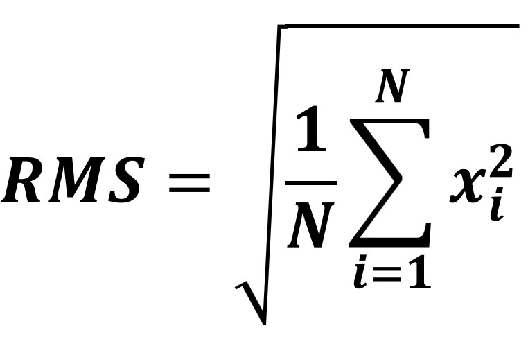
1. RMS = Sqrt(1/N(i12 + i22 + i32 + i42 + … + iN2 ); Root Mean Square For N Sample Currents i
Picture: RMS Equation; Discrete Form
The RMS is a type of average value or average magnitude that is particularly useful for quantifying the overall size of a set of numbers or a time-varying signal, regardless of its sign.
Unlike the simple arithmetic mean (average), which can be very small for a set of numbers with both positive and negative values (for example, the average of 5, -7, 10, and -4 is 1, which is smaller than any of the values),
the RMS calculation provides a magnitude that is more indicative of the true average magnitude.
In that example, the RMS is approximately 6.89.
Because the RMS calculation inherently squares all values, it is especially effective for cyclic data sets like sine waves.
This makes it invaluable in fields like AC power computations, where it allows AC voltages and currents to be expressed as a DC equivalent that produces the same amount of power, since power (P) is proportional to the square of the current (I2).
Approximate RMS of a Sinusoidal Curve
Consider the simple periodic sinusoidal motion of current.
A plot of current plotted for one cycle (one period) would show a sine curve as shown in the picture below.
In the context of periodic motion, 1 period is exactly like going around a circle once, completing a full 360 degree revolution, or 2π radians.
Picture: Current (i) Sine Wave
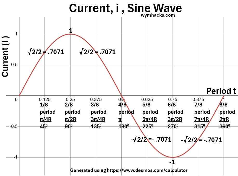
Let’s divide 1 full cycle (one period) into 8 equal sections.
On the x axis of the chart above, I’ve stated this in 1/8 periods but also in Radians (2πR = 360 degrees) and degrees.
The current, period values from the chart are
- (0t,0),
- ((1/8)t,√2/2),
- ((2/8)t,1)
- ((3/8)t,√2/2)
- ((4/8)t,0)
- ((5/8)t,-√2/2)
- (6/8t,-1)
- ((7/8)t,-√2/2)
- ((8/8)t,0)
We want to take the Root Mean Square of the signal which means we want to take the square root of the average of the squares of the y values (the current or i).
1. RMS = Sqrt(1/N(i12 + i22 + i32 + i42 + … + iN2 ); Root Mean Square For N Sample Currents i
For our example,
iRMS = SQRT (1/8 ( 02 + (√2/2)2 + 12 + (√2/2)2 + 02 + (-√2/2)2 + -12 + (-√2/2)2 ) )
iRMS = SQRT (1/8 ( 0 + .5 + 1 + .5 + 0 + .5 + 1 + .5 ) ) = SQRT (.5) = .70711
or
iRMS = .70711 = √2/2
Since the maximum sine value from our example graph is 1 , we can describe as I “RMS” or I “Effective” as follows:
2. IRMS = IEFF = (√2/2) IMAX
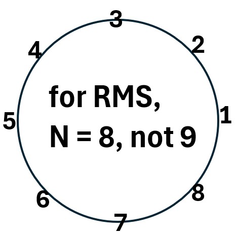
Notice that in the graph there are actually 9 discrete points shown, but the first is equal to the last, so we cant include both.
This is obvious when you look at the cyclic nature of the points in the picture below where you do not count point 1 twice (i.e. point 1 = point 9)
Picture: Quarter Period Points For a Sine Wave
Now, let’s derive a more accurate (mathematically perfect) RMS equation for smooth continuous functions (like sine waves).
RMS Equation (Continuous Form)
Recall the discrete form of the RMS equation.
Picture: RMS Equation; Discrete Form
3. 
The discrete form of the RMS equation becomes more accurate with a higher number of data points.
If we had infinite points, we would have our most accurate RMS vale, so let’s do this in the context of our sine wave (see picture below)
Picture: Sine Wave (for current); Showing a Differential period section dt
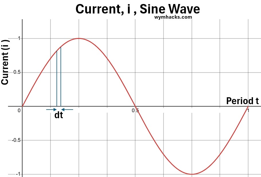
This sine wave can be defined as
4. i(t) = IMsin(t+ϕ ) ; current i sine wave equation
where
- i(t) : Instantaneous Current ; Amperes (A); The current at any specific point in time, t.
- IM : Maximum (Peak) Current; Amperes (A); The maximum value the current reaches in either the positive or negative direction (the amplitude of the wave).
- ω Angular Frequency; Radians per second (rad/s); The speed at which the current is cycling.
- It is related to the frequency f by the formula: ω=2πf.
- t : Time; Seconds (s)
- ϕ: Phase Angle (or Phase Shift); Radians (rad) or Degrees ; The offset of the sine wave from the origin (t=0). It indicates the starting position of the wave.
Assume the phase angle ϕ = 0.
5. i(t) = IMsin(t)
We can express equation 3 (the discrete form of the RMS) in its continuous form ( its most accurate form ) when the number of samples are infinite (N → ∞ ):
6. 
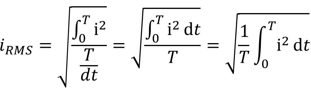
This square root of integrals form is just a reformulation of the discrete RMS formula written in summations of infinitely small sections (i.e. integral) where
- ∫i2dt is an infinite sum of squared current values over infinitely small periods and
- T/dt is equal to an infinite number of sample points.
6. iRMS = SQRT (1/T∫i2dt) evaluated from T = 0 to T ; RMS for continuous function (a sine wave in this example).
Well, we’ve come too far to just stop here!
Lets solve for the continuous RMS of the sine wave function i(t) = IMsin(t)