Introduction
In this post we’ll explore the properties of sine and cosine functions.
These are trigonometric (from the Greek trigōnon: meaning “triangle” and metron: meaning “measure) functions which most of us are introduced to via the mnemonic:
SohCahToh (o = opposite, h = hypotenuse, a = adjacent).
Picture: Right Triangle Trig Definitions

For right triangle where 0 < θ < 900
(1) a2 + b2 = c2 ; Pythagorean Theorem
(2) sin(θ) = opposite/hypotenuse = a/c
(3) cos(θ) = adjacent/hypotenuse = b/c
(4) tan(θ) = opposite/adjacent = a/b
note: there are other, broader, definitions we’ll review later.
All other trigonometric functions and identities (like tangent and many others) are defined and derived from the sine and cosine functions.
Who cares ?, you might ask.
You should because they help you (and other curious and creative people) understand the way the world works.
Sine and Cosine are the fundamental building blocks of all periodic phenomena in nature, making them indispensable tools in fields like physics and engineering.
In Electrical Engineering (EE), they are the mathematical language used to describe Alternating Current (AC), which powers homes and industry worldwide.
Specifically, the sinusoidal (sine/cosine) wave models the voltage and current that vary smoothly over time, allowing engineers to
- analyze and manipulate complex circuits,
- understand power transmission, and
- design everything from simple filters to advanced communication systems.
Their use is crucial for the techniques of phasor analysis, Fourier analysis, and signal processing, which are foundational to the discipline.
Read this nice article: Intuitive Understanding of Sine Waves – betterexplained.com
Ok, let’s start with a little history, and then dive into the definitions and properties of sine and cosine.
History
Check out Appendix 1 for much more detail!
The history of the sine function is a transition from an arc (line defined by two points on the circumference of a circle) length to a dimensionless ratio.
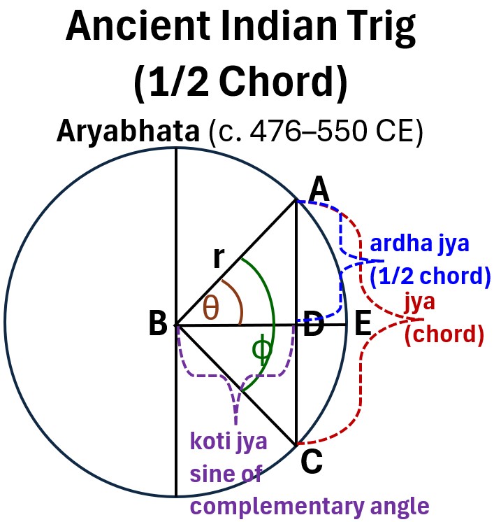
Initially, Greek mathematicians/astronomers, like Hipparchus and Ptolemy (c. 100 CE), defined it geometrically using the length of a chord subtended by a central angle in a circle (e.g. see chord AC and angle ɸ in the picture below) .
Around the 5th century CE,
- Indian mathematicians, most notably Āryabhaṭa, simplified this to the half-chord or ardha jya (which became the Latin sinus),
- essentially defining it as the side opposite an angle in a right triangle inscribed in a circle of a fixed radius.
Over the Islamic Golden Age (c. 9th–13th centuries),
- the functions were developed systematically and applied widely, along with the co-functions.
Picture: Sine and Cosine Historical Roots are in the Chord and 1/2 Chord of a Circle
Finally, European mathematicians like Euler (18th century) formalized the concept by
- setting the circle’s radius to one,
- establishing sine and cosine as the dimensionless ratio of the side of a right triangle to the hypotenuse,
- which is the definition we use in modern analysis.
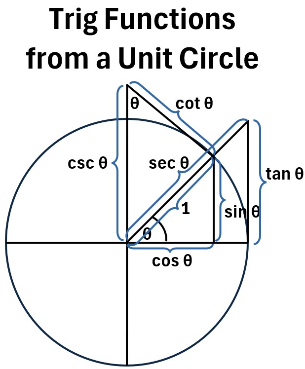
Picture: Trig Functions from a Unit Circle
Unit Circle Trigonometry
Consider a unit circle with a radius of 1 centered at the origin (0,0):
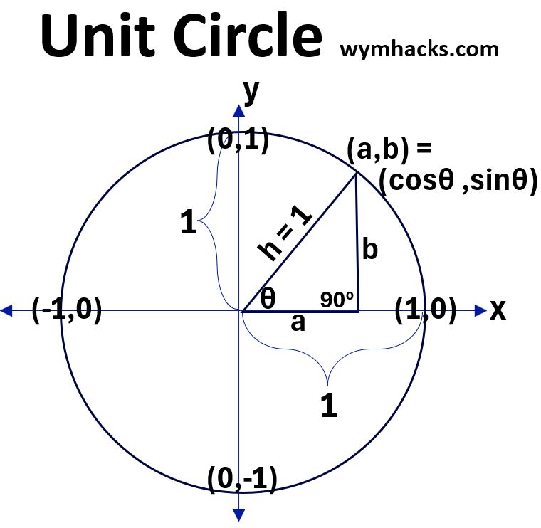
(5) On a unit circle, by definition, every point on the circumference will have coordinates (a,b) = (x,y) = (cosθ,sinθ)
(5a) x = cosθ
(5b) y = sinθ
where,
- angle θ is defined as 0 for the x axis line that intersects the unit circle at (1,0)
- and θ increases counterclockwise all the way around the circle back to 0 degrees (or 360 degrees).
We can use a right triangle in the first quadrant of the unit circle to establish more broad definitions for the trigonometric functions.
Unit Circle Trigonometry – For All Four Quadrants
The definition of sine and cosine on the unit circle is consistent across all four quadrants of a cartesian plane:
- cos θ is the x-coordinate of the point on the circle.
- sin θ is the y-coordinate of the point on the circle.
While you use a right triangle for the first quadrant, the key to the other quadrants is understanding
- symmetry and the reference angle θR
to determine the magnitude of the value, and
- the coordinate system
to determine the sign of the value.
Unit Circle Trigonometry – Sign of (x,y) Values
The unit circle is overlaid on the Cartesian coordinate plane, which dictates the sign of the x and y coordinates in each quadrant.
Since cos θ = x and sin θ = y, the signs of x and y directly determine the signs of the functions.
Unit Circle Trigonometry – Magnitude (x,y) Values
Refer to the drawing below.
Picture: Unit Circle with Right Triangles in Each Quadrant
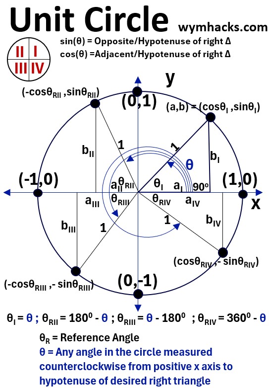
For any angle θ, starting at the positive x axis and extending into Quadrants I, II, III, or IV, you can create a corresponding right triangle.
- Note, the quadrants begin at the top right (I) and go counterclockwise to quadrants II, III, and IV.
This triangle is formed by the terminal side of θ , the x-axis, and a vertical line from the point on the circle to the x-axis.
The reference angle θRII or RIII or RIV is the positive acute angle between the terminal side of θ and the closest part of the x-axis.
- θI = θ ; Quadrant 1 Angle
- θRII = 1800 – θ ; Quadrant 2 Reference Angle
- θRII = 0 – 1800 ; Quadrant 2 Reference Angle
- θRII = 3600 – θ ; Quadrant 2 Reference Angle
The trigonometric value (magnitude only) for any angle θ is the same as the value for its reference angle θ , which is always in Quadrant I.
So, we can now define the trigonometric functions for all angles (i.e. we are not confined to right triangles where θ must be >0 degrees and < 90 degrees).
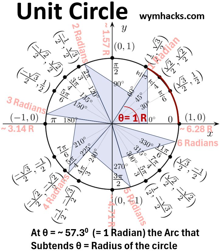
In the picture below, I show the (cosine, sine) values for select points all around the unit circle.
Notice that the values in quadrants II, III, and IV have the same magnitudes as the values in Quadrant I.
Picture: Unit Circle With Trigonometric Values
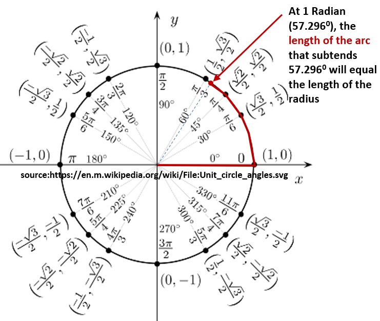
In the diagram above, the angle values π/6, π/4, π/3, π/2, 2 π/3 etc. are in Radians where 2π Radians = 3600= one rotation around the circle.
The Radian as an Angle Measure
If we
- start the radius in the positive horizontal position and
move it counterclockwise until θ = 1 Radian, then
the length of the arc that subtends θ will equal the length of the radius
- The arc of 1 Radian (equal to the radius length) is traced out in red in the picture above
(6) In fact, the definition of a Radian is the ratio of the arc length to the radius of a circle.
Subtend means to be opposite to and extend from one side to the other of something.
- For example, in the Unit Circle above, the circle arc from point (1,0) to point (sqrt(3)/2 , 1/2) subtends the angle of 300
Moving from the horizontal positive radius line of the Unit Circle in a counterclockwise direction:
- θ = 300 = π/6 Radians = π/6 R
- θ = 450 = π/4 R = ~ .785 R
- θ = ~ 57.30 = 1 Radian
- θ = 600= π/3 R = ~ 1.05 R
- θ = 900 = π/2 R
- θ = 1800 = π R
- θ = 2700 = 3π/2 R
- θ = 3600 = 2πR
See Appendix 2 for more on the Radian.
Sine and Cosine Wave
In this section we’ll generate the sine and cosine graphs using the Unit Circle.
The idea here is we are translating a 2 dimensional position on the unit circle into a one dimensional position on a graph.
(7) The sine wave’s characteristic shape is generated by plotting the vertical displacement (the y axis of the unit circle) against the angle of rotation (or time).
For the Unit Circle (see the picture below), start with a point on the circumference at (cosθ,sinθ) = (1,0) and rotate it counterclockwise.
Picture: Sine Graph from The Unit Circle
![]()
Plotting the associated vertical displacement versus the angle of rotation (shown in radians in the graph) produces the sine wave shown above.
(8) Similarly, the cosine wave’s characteristic shape is generated by plotting the horizontal displacement (the x axis of the unit circle) against the angle of rotation (or time).
If we plot the displacement and associated angle for each counterclockwise rotating point, we’ll get the cosine wave shown in the picture below
Picture: Cosine Graph from The Unit Circle
In the picture above, I show the position/angle graph vertically below the unit circle so its clear that we are simply plotting the horizontal displacements and their associated angles.
I’ve then just rotated the graph so we can compare the sine and cosine graphs more easily. You can see they do look very similar.
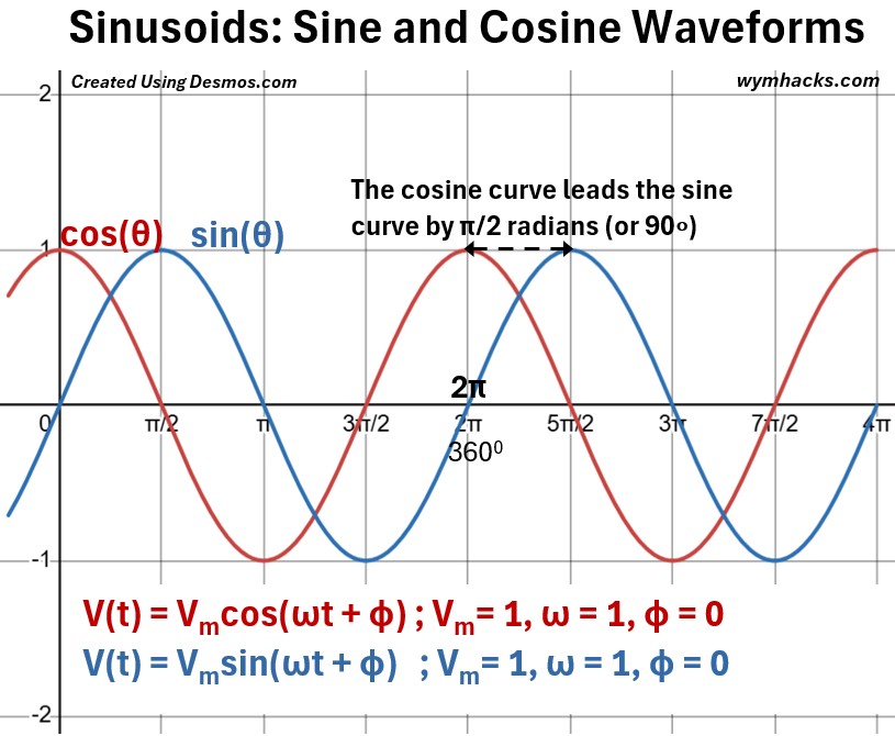
The graph below combines the sine and cosine curves on the same axis.
Picture: Sine and Cosine Waveforms
![]()
The cosine and sine waves have the exact same shape and period (distance between peaks or troughs), but they are shifted horizontally from one another by π/2 radians or 90°.
They are often referred to as being π/2 radians or 90° out of phase.
This means you can transform one into the other by simply shifting it horizontally:
(9) cos(θ) and sin(θ) are out of phase by π/2 rad or 90°
(9a) cos(θ) = sin(θ + π/2)
(9b) sin(θ) = cos(θ – π/2)
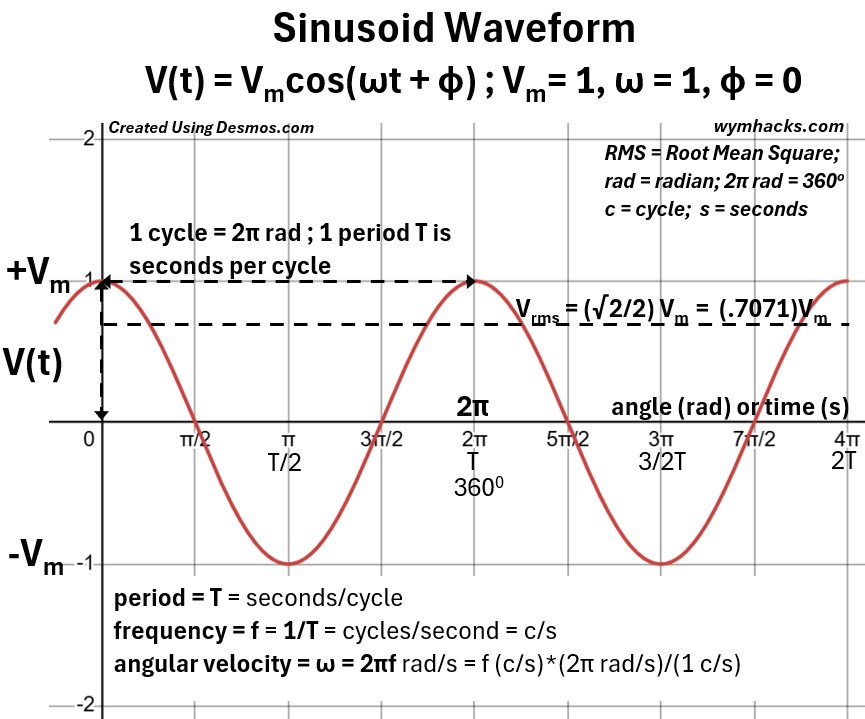
Sinusoid Waveform General Characteristics
The chart below shows the main characteristics of a sinusoid wave.
Picture: Sinusoid Waveform Characteristics

The following terms describe the characteristic shape and properties of a transverse wave where the oscillations are perpendicular to the propagation.
Crest (in meters)
(10) The crest is the highest point of the wave, representing the maximum positive displacement from the 0 position (the equilibrium or rest position).
Trough (in meters)
(11) The trough is the lowest point of the wave, representing the maximum negative displacement from the 0 position (the equilibrium or rest position).
Amplitude (in meters)
(12) The amplitude is the maximum distance or height a point on the wave moves from its central equilibrium position to the crest or trough.
Wavelength (λ; in meters)
(13) The wavelength is the spatial length of one complete wave cycle, measured as the distance between two successive identical points (e.g., crest to crest or trough to trough).
Cycle (dimensionless)
(14) One cycle is one complete repetition of the wave’s shape and motion, equivalent to the distance of one wavelength.
Frequency (f; in Hertz = cycles/second)
- The frequency f is the measure of how often a repeating event occurs.
- (15) f = the number of cycles or full repetitions of a wave or oscillation that occur in a specific unit of time.
- SI Unit: The hertz (Hz), which is defined as one cycle per second = 1/s
- I like to show this as cycles/second and not just 1/sec to stress the true meaning of the term
Period (T; seconds/cycle)
- The period T is the measure of the time it takes for one cycle to occur.
- (16) The period T is The time interval required for a single, complete cycle, oscillation, or vibration to take place.
- SI Unit: The second (s) as in seconds/cycle
- Relationship to Frequency: Frequency and period are reciprocals of each other.
- (17) T = 1/f ; f = 1/T
Dimensionless Quantities
You’ll notice that cycles are not given units of measure. They are considered dimensionless in the SI system.
In the International System of Units, cycles are dimensionless because they are defined as counts.
- A Cycle is a count of one repetition, which is treated as the number one.
Note that the Radian is also dimensionless.
- A radian is the measure of an angle where the arc length is exactly equal to the radius of the circle.
- It is dimensionless because it is defined as the ratio of two lengths: angle in radians = arc length/radius
Circular Motion Parameters
You can read my post: Rotational Motion Variables for a detailed study of the key variables describing rotational (circular) movement.
In this post I’ll simply provide the picture below and provide the basic definitions for the rotational variables:
- θ = Angular Displacement
- ω = Angular Velocity
- α = Angular Acceleration
Picture: Circular Motion Parameters
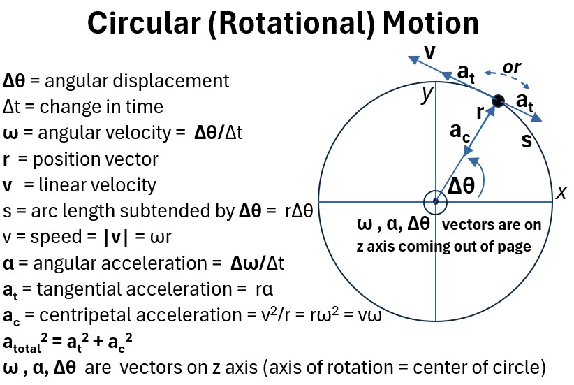
θ: Angular Displacement
Angular displacement is the change in the angular position of a rotating object, measured in radians, with its vector direction defined along the axis of rotation by the right-hand rule.
The defining relationship that links angular displacement θ to the distance traveled along the arc s is
(18) s = r Δθ ; magnitude of arc length
- s = arc length (the distance covered along the circular path)
- r = radius of the circular path
- θ = angular displacement (the angle subtended by the arc s) measured in radians
ω: Angular Velocity
Angular velocity is a measure of the rate of change of angular displacement of a rotating body.
- It quantifies how fast an object is rotating or revolving.
- ω = dθ/dt
- Scalar Magnitude: It is the rate at which the angle changes, measured in radians per second
- Vector Direction: Its direction is specified along the axis of rotation using the right-hand rule.
For rotation about a fixed axis, the magnitude of the linear velocity vt is
(19) vt = rω ; magnitude of linear (tangential) velocity (speed)
- vt = magnitude of linear velocity = tangential speed
- ω = angular velocity
- r = radius
α: Angular Acceleration
Angular Acceleration α is a measure of the rate of change of angular velocity of a rotating body.
It quantifies how quickly an object’s rotation is speeding up or slowing down.
- α= dω/dt = d2θ/dt2
- Scalar Magnitude: Measured in radians per second squared
- Vector Direction: Its direction is along the axis of rotation.
For rotation about a fixed axis, the magnitude of the tangential acceleration is
(20) at = rα ; magnitude of tangential acceleration
- α = angular acceleration
- r = radius
Voltage and Current Waveform Characteristics
We know what the equations look like for AC voltage and current.
Now lets see how the various variables affect the shapes of the sinusoids.
In the first graph below, we see how the cosine curve leads the sine curve by π/2 radians (or 90 degrees).
- The relationship between the two waveforms is determined by which one reaches a characteristic point—like zero (crossing the axis) or its positive maximum— first in time (reading the graph from left to right).
- Leading: The waveform that reaches its maximum or zero value at an earlier time (to the left on the time axis) is said to be leading the other.
- Lagging: The waveform that reaches the same point at a later time (to the right on the time axis) is said to be lagging behind the other.
Picture: Sinusoids: Sine and Cosine Waveforms
In the graph below, for the cosine version of the voltage, we can define a few more variables:
- Root Mean Square Voltage = Vrms = (sqrt(2)/2)Vrms
- See my blog: RMS (Root Mean Square) of a Sinusoid for how to derive it
- Relative to the cosine wave, Vrms is a horizontal line with a magnitude about 70.71% of the maximum voltage.
Voltage Sinusoid Waveform – Vrms, Period, Frequency, and Angular Velocity
From the voltage sinusoid graph above we can also define the following:
- 1 cycle is the distance from peak to peak (or trough to trough)
- 1 cycle = 2π radians
- 1 period = T = seconds/cycle
- The frequency = f = 1/T = cycles/second = Hertz
- Angular velocity = ω = 2πf = 2π/T = radians/s
- In circuit analysis, Electrical Engineers will sometimes call ω the angular frequency which is not really correct.
- ω “contains” the frequency term f but it is the angular velocity , not the frequency.
In the graph below, we vary Vmax , the amplitude, of the voltage equation.
Voltage Sinusoid Waveform: Vmax (Amplitude) Variation
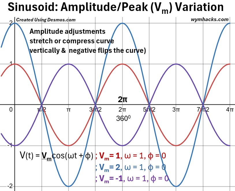
In the graph above, you can see that the amplitude varies as Vmax is changed from 1 to 2 to -1.
Amplitude adjustments stretch or compress the curve vertically and a negative value “flips” the curve.
Lets tweak the angular velocity (sometimes called frequency) and observe the results in the graph below.
Voltage Sinusoid Waveform: Angular Velocity ω (Frequency) Variation
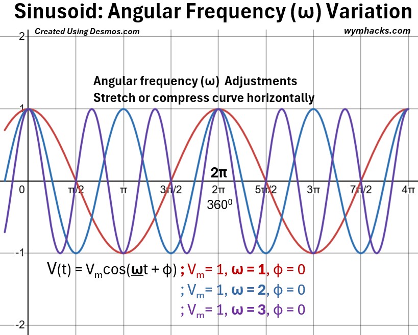
As the angular velocity ω is increased from 1 to 3, the curve is compressed horizontally (and vice versa for deceasing ω).
We’ve had the phase angle Φ zeroed out in the graphs above.
The graph below shows the changes when Φ goes from 0 to +π/2 and to – π/2.
Voltage Sinusoid Waveform: Phase Angle Φ Variation
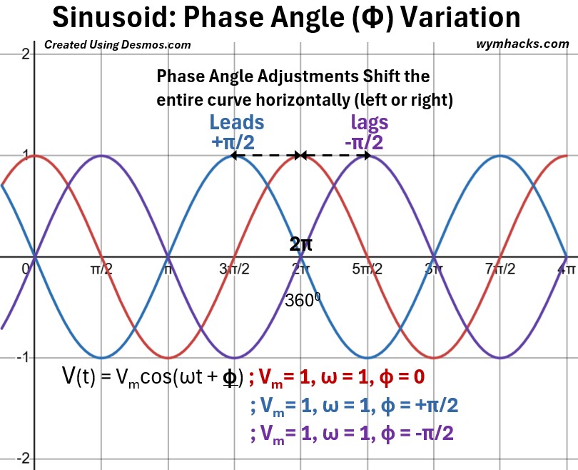
From the graph above we see that phase angle Φ adjustments shift the entire curve horizontally.
- Addition of – π/2 “pushes” the baseline (the red Φ = 0 curve) curve to the right.
- The resultant curve (the purple line) now “lags” the red curve
- Addition of π/2 “pushes” the baseline (the red Φ = 0 curve) curve to the left.
- The resultant curve (the blue line) now “leads” the red curve
Three Phase AC Voltage Sinusoids
Picture: 3 Phase AC Voltage Sinusoids
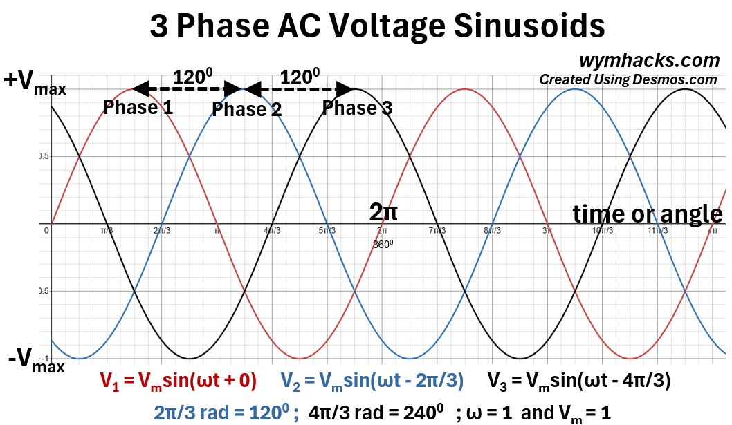
This graph illustrates a balanced three-phase voltage system, which is the standard method for distributing electrical power in modern electrical grids.
It features three distinct sinusoidal waves V1 (red), V2 (blue), and V3 (black)— all oscillating around a central zero-axis with the same peak amplitude (Vmax) and frequency.
The defining characteristic of this graph is the phase displacement; each wave is mathematically offset from the others by exactly 1200 (2π/3 radians).
This creates a sequential “staggered” effect where V1 peaks first, followed by V2, and finally V3, ensuring that power is delivered in a continuous, overlapping stream rather than in single pulses.
Phase Separation
The equations (see picture above)
- V1 = Vmsin(ωt),
- V2 = Vmsin(ωt – 2π/3), and
- V3 = Vmsin(ωt – 4π/3)
show that the curves are perfectly spaced across one full rotation (3600 or 2π).
Instantaneous Sum of Zero
One of the most critical properties of this balanced system is that at any vertical slice of the graph (any moment in time), the sum of the three voltages equals zero (V1 + V2 + V3 = 0).
This allows for efficient grounding and neutral-wire configurations in power systems.
Constant Power Delivery
While a single sine wave (single-phase) drops to zero power twice every cycle, the sum of power in a three-phase system is constant.
As one voltage curve falls toward the zero line, the other two are at high enough magnitudes to maintain a steady flow of energy.
Directional Rotation
The sequence of the peaks (red → blue → black) establishes a “phase sequence.”
In an industrial motor, this specific timing is what determines the physical direction in which the motor’s shaft will rotate.
Approximating sin(x) and cos(x) Using Infinite Sums
The Maclaurin series provides a way to approximate trigonometric functions like sin(x) and cos(x) by expressing them as infinite sums of polynomial terms.
Because these functions are smooth and infinitely differentiable, they can be represented by power series centered at zero.
- The series for sin(x) consists only of odd-numbered powers, reflecting its nature as an “odd function” that is symmetric about the origin, while
- the series for cos(x) contains only even-numbered powers, consistent with its “even function” symmetry across the y-axis.
In practical applications, we rarely use the infinite sum; instead, we use a “Taylor polynomial” by cutting the series off after a few terms.
As more terms are added to the calculation, the polynomial “hugs” the curve of the actual sine or cosine wave over a wider range, providing an increasingly accurate approximation that is essential for calculator algorithms and complex physics simulations.
The Series Equations
The mathematical representations for these approximations are:
(28) sin(x) = ∑n=0–>∞ [(-1)nx(2n+1)/(2n + 1)!]
(29) cos(x) = ∑n=0–>∞ [(-1)nx(2n)/(2n)!]
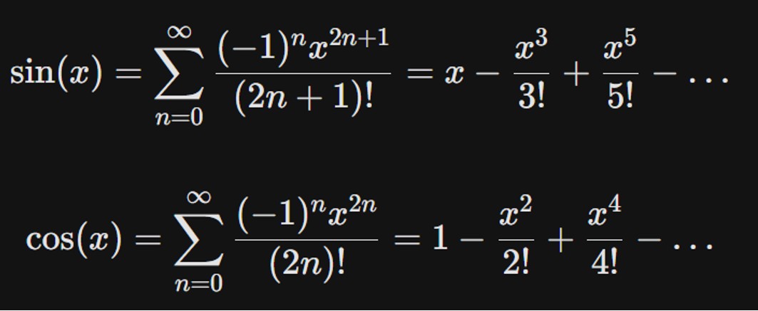
Alternating Signs
Both series flip between positive and negative terms, which allows the polynomial to “bend” back and forth to mimic the oscillating nature of a wave.
Factorial Denominators
The denominators (3!, 5!, etc.) grow extremely quickly, meaning that higher-power terms become very small, ensuring the series converges to the true value of the function.
Small Angle Approximation
For very small values of x, we can ignore the higher-order terms, which is why sin(x) ≈ x is a common and useful simplification in physics.
Picture: sin(x) Maclaurin Series Charted with Increasing Terms

Simple Harmonic Motion Equation
Sine and cosine can also be defined as solutions to the Simple Harmonic Motion (SHM) equation.
The solution can be expressed in one of three formats:
- x(t) = Asin(ωt + Φ1) + Bcos(ωt + Φ2) ; Sine & Cosine Form of General Solution to the Simple Harmonic Motion Equation
- x(t) = Cccos(ωt + Φc) ; Cosine Form of General Solution to the Simple Harmonic Motion Equation
- x(t) = Cssin(ωt + Φs) ; Sine Form of General Solution to the Simple Harmonic Motion Equation
For these to make sense , we need to start with the concept of simple harmonic motion (SHM) and the equation that describes it.
So, we’ll start with understanding SHM and then do the trigonometry and algebra needed to show how the equations above satisfy it mathematically.
Simple Harmonic Motion Equation
So, we need to start with Hooke’s Law which I discuss also in my article: Work and Energy
Consider the setup shown in the picture below where a block of mass m is attached to a spring which is attached to a wall.
From a starting position x= 0, the mass is pulled (spring is stretched) to position x.
Picture: Hooke’s Law
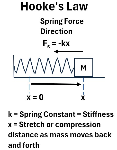
In this setup, Hooke’s Law states that the restoring force (Fs) exerted by the spring is directly proportional to the displacement (x) of the block from its equilibrium position.
(30) Fs = -kx
- k (Spring Constant): This represents the stiffness of the spring; a higher k means a stronger pull for the same distance.
- The Negative Sign (-):
- This is the most critical part of the drawing.
- It indicates that the force is always a restoring force—since you stretched the block to the right (+x), the spring pulls back to the left (-Fs), always trying to return the mass to x = 0.
To derive the equation for Simple Harmonic Motion (SHM), we apply Newton’s Second Law.
(31) F = at
Newton’s Second Law states that the
- acceleration (a) of an object is directly proportional to the
- net force acting on it (F) and
- inversely proportional to its mass (m)
The only horizontal force acting on the mass (ignoring friction) is the spring force, -kx.
S0,
(32) F s = -kx = at
Since acceleration (a) is the second derivative of position with respect to time (see my article The Derivative to remember why),
(33) Acceleration = a = d2x/dt2
Substituting (33) into (32),
(34) Fs = -kx = md2x/dt2
Moving all the terms to one side we get
(35) d2x/dt2 + (k/m)x = 0 ; Simple Harmonic Motion Equation
We can express k/m as ω2
where ω is our old friend the angular frequency (it’s really an angular velocity with units of radians/second).
(36) k/m = ω2 ; See the details of why this is true in Appendix 3.
so (35) can be expressed with ω as well
(37) d2x/dt2 + (ω2)x = 0 ; Simple Harmonic Motion Equation
- This is a “second-order differential equation”.
- It says that the more you stretch something, the harder it snaps back.
- In physics, it’s formally known as the Equation of Motion for a Simple Harmonic Oscillator
General Solution to the Simple Harmonic Motion (SHM) Equation
The expression
(38) x(t) = Asin(x) + Bcos(x) ; Sine and Cosine Form of the General Solution to the Simple Harmonic Motion Equation
is the general solution to the SHM (equation 37).
Let’s prove it (after we do a little prep. work).
We need some math tools to do this, so let’s start there.
Math Tools
We know that (see my articles: Geometry and Trigonometry Rules and Sum and Difference Angle Formula Proofs )
(39) sin(α + β) = sinα cosβ + cosα sinβ
(40) cos(α + β) = cosα cosβ – sinα sinβ
(41) cos2θ + sin2θ = 1 ; Pythagorean Identity
and (see my article: The Derivative)
(42) d/dx(sin(x)) = cos(x)
(43) d/dx(cos(x)) = -sin(x)
General Solution Equation
Let’s re-write equation (38) understanding that we can express x (an angle) as
(44) x = ωt + Φ where
- ω (Angular Frequency): This measures the speed of the oscillation in terms of rotation (rad/s).
- t (Time): The independent variable representing the moment in time you are measuring. Measured in seconds (s).
- ωt (Phase): It is the “angle” the oscillator has swept out since it started its current cycle.
- Φ (Phase Constant or Phase Shift):This defines the initial state of the system at exactly t = 0.
So (38) becomes
(45) x(t) = Asin(ωt + Φ1) + Bcos(ωt + Φ2) ; Sine and Cosine Form of the General Solution to the Simple Harmonic Motion Equation
- x(t): The instantaneous displacement.
- This is the final position of the object at any given time t after combining both waves.
- A and B: The amplitudes of the individual components.
- A is the maximum “reach” of the sine wave, and B is the maximum “reach” of the cosine wave.
- ω: The angular frequency.
- Notice that ω is the same for both parts.
- This means both components are “beating” or vibrating at the exact same speed.
- Φ1 + Φ2: The phase constants.
- These tell you that the sine wave and the cosine wave didn’t necessarily start at the same time or place.
- The difference between them Φ1 – Φ2 is called the phase difference.
Proving the General SHM Solution Equation
Lets first prove that equation (45) is a solution to the SHM equation (37).
So let’s start with equation (45), re-written below, and take the first and second derivatives.
(45) x = Asin(ωt + Φ1) + Bcos(ωt + Φ2)
(46) dx/dt = d/dt[Asin(ωt + Φ1) + Bcos(ωt + Φ2)]
(47) dx/dt = Aωcos(ωt + Φ 1 ) – Bωsin(ωt + Φ 2 )
(48) d2x/dt2 = -Aω2sin(ωt + Φ1) – Bω2cos(ωt + Φ2)
(49) d 2 x/dt 2 = – ω 2 [Asin(ωt + Φ 1 ) + Bcos(ωt + Φ 2 )]
The bracketed expression on the RHS of (49) is equal to the RHS of (45).
So,
(50) d2 x/dt2 = – ω2[Asin(ωt + Φ 1 ) + Bcos(ωt + Φ 2 )]
(51) d2x/dt2 = – ω2x = Equation (37) = Simple Harmonic Motion Equation
So, we’ve proven that “x = Asin(ωt + Φ1) + Bcos(ωt + Φ2) ” is a solution to the Simple Harmonic Motion Equation.
Q.E.D (Quod Erat Demonstrandum, which literally translates to: “Which was to be demonstrated.” i.e. we proved it)
Expressions for the General Solution to the Simple Harmonic Motion Equation
The general solution to the Simple Harmonic Motion Equation can be expressed in three ways
- The Sine & Cosine Form: We’ve described and proven this above.
- The Sine Form: Expressed as a single Amplitude and Phase equation with the sine function.
- The Cosine Form: Expressed as a single Amplitude and Phase equation with the cosine function.
These equations and their associated coefficients and phase angles are summarized below.
See Appendix 4 for the detailed derivations.
Sine & Cosine Form of the General Solution to the Simple Harmonic Motion Equation
(45) x(t) = Asin(ωt + Φ1) + Bcos(ωt + Φ2) ; Sine & Cosine Form of General Solution to the Simple Harmonic Motion Equation
Cosine Form of the General Solution to the Simple Harmonic Motion Equation
(52) x(t) = Cccos(ωt + Φc) ; Cosine Form of General Solution to the Simple Harmonic Motion Equation
(52a) Cc = sqrt(M2 + N2) ; Coefficient Cc for Cosine Form of General Solution to the Simple Harmonic Motion Equation
(52b) M = – CcsinΦc = (AcosΦ1 -BsinΦ2) ; Coefficient M for Cosine Form of General Solution to the Simple Harmonic Motion Equation
(52c) N = CccosΦc = (AsinΦ1 +BcosΦ2) ; Coefficient N for Cosine Form of General Solution to the Simple Harmonic Motion Equation
(52d) Φc = arctan [(BsinΦ2 – AcosΦ1)/ (AsinΦ1 +BcosΦ2) ] ; Phase angle Φc for Cosine Form of General Solution to the Simple Harmonic Motion Equation
Sine Form of the General Solution to the Simple Harmonic Motion Equation
(53) x(t) = Cssin(ωt + Φs) ; Sine Form of General Solution to the Simple Harmonic Motion Equation
(53a) Cs = sqrt(M2 + N2) ; Coefficient Cs for Sine Form of General Solution to the Simple Harmonic Motion Equation
(53b) M = CscosΦs = (AcosΦ1 – BsinΦ2) ; Coefficient M for Sine Form of General Solution to the Simple Harmonic Motion Equation
(53c) N = CssinΦs = (AsinΦ1 + BcosΦ2) ; Coefficient N for Sine Form of General Solution to the Simple Harmonic Motion Equation
(53d) Φs = arctan [ (AsinΦ1 + BcosΦ2) /(AcosΦ1 – BsinΦ2) ] ; Phase angle Φs for Sine Form of General Solution to the Simple Harmonic Motion Equation
Summary
The general solution to the Simple Harmonic Motion Equation can take three forms:
(45) x(t) = Asin(ωt + Φ1) + Bcos(ωt + Φ2) ; Sine & Cosine Form of General Solution to the Simple Harmonic Motion Equation
(52) x(t) = Cccos(ωt + Φc) ; Cosine Form of General Solution to the Simple Harmonic Motion Equation
(53) x(t) = Cssin(ωt + Φs) ; Sine Form of General Solution to the Simple Harmonic Motion Equation
Appendix 1: History of Sine and Cosine
Greeks and Indians – Chords and Half Chords
The ancient Egyptians (roughly 4700 years ago) and Babylonians (roughly 3800 years ago) used ratios of triangles for construction and measurement.
- The Egyptians used the concept of inverse slope or “seked” in the building and construction
- Evidence of Babylonian’s use of triangle geometry is the cuneiform tablet known as Plimpton 322 (c. 1800 BC).
Historians think that the precursors to sine and cosine started with the work of the ancient Greek Hipparchus of Nicaea (c. 190 – c. 120 BC; about 2215 years ago) who gets the nice title “father of trigonometry”.
He related chords in circles to the angles they subtended (i.e. heights of right angle triangles and the acute angle opposite them).
These concepts were notably systematized by Claudius Ptolemy (c. 100 – c. 170 CE) in his Almagest.
- Tabulations: Chord of θ was a length subtending a central angle θ in a circle of a fixed, large radius r.
The crucial conceptual leap occurred with Indian astronomers (notably Aryabhata (c. 476–550 CE)) who replaced the full chord with the half-chord—a line segment equal to half the chord of the doubled angle, or 1/2 chord(2θ) .
This half-chord, known as ardha jya, is mathematically and geometrically equivalent to the modern definition of rsinθ.
He also defined the cosine (ko-jyā, short for koti-jyā).
- The koṭi-jyā referred to the length of the side adjacent to the angle θ in a right-angled triangle inscribed within a circle of a fixed radius r.
- This is the complement of the sine (or jyā).
Picture: Ancient Indian 1/2 Chord in a Circle Concept (ardha jya and koti jya)
Kerala School (1340 – 1425 CE); ~ 685 years ago
We will cover this later in the post but, defining sine and cosine using an infinite power series is considered a more rigorous and fundamental definition than the initial geometric definition based on a right-angled triangle or a circle (the “half-chord” definition).
Amazingly, Indian mathematicians of the Kerala School (e.g., Madhava, c. 1340–1425 CE) pioneered infinite series expansions for trigonometric functions.
Mādhava developed and used methods that were essentially a form of calculus—specifically, an early understanding of limits, infinitesimals, and infinite summation (integration)—to derive these exact infinite series expansions for sine and cosine.
He achieved these results about 300 years before the formal and generalized discipline of calculus was developed by Isaac Newton and Gottfried Leibniz in Europe.
Arab and Persian Mathematicians (c. 9th–13th centuries: 801 to 1301 AD)
Arab and Persian Mathematicians adopted this method, using the half-chord alongside its complement, the cosine (cos(θ) = sin(90° – θ)), and treated them as lengths for sophisticated spherical astronomy.
- Al-Khwārizmī (Persian) 9th Century: Compiled some of the earliest sine and cosine tables in the Islamic world.
- Al-Battānī (Arab) 9th-10th Century: Introduced the systematic use of the sine and tangent
- al-Buzjani (Persian) 10th Century: Introduced the secant and cosecant functions. Proved the Law of Sines for spherical triangles. Created highly accurate sine tables.
- al-Tusi (Persian) 13th Century: Wrote the first book to treat trigonometry as an independent branch of pure mathematics, separate from astronomy.
Europe
- 1464: The First Modern Treatise: German astronomer and mathematician Regiomontanus (Johannes Müller, 15th century) wrote De Triangulis Omnimodis (On Triangles of All Kinds) in 1464.
- The Complete Set of Functions: Georg Joachim Rheticus (16th century) published the first European tables to include all six standard trigonometric functions sin,cos,tan,cot,sec,csc.
- He also spent decades creating monumental, highly accurate tables (some up to 20 decimal places).
- 1595: Coined the Term “Trigonometry”: The German mathematician Bartholomäus Pitiscus is credited with first using the term “Trigonometria” in his 1595 publication.
1665-1685: Newton and Leibniz
- advanced the study of trigonometry by establishing the foundation of calculus, which allowed sine and cosine to be treated as analytic functions rather than just geometric lengths.
- They were the first in Europe to systematically use the infinite power series (like the Maclaurin series) to define these functions, essentially transforming trigonometry from a geometric discipline into a core part of modern mathematical analysis.
- This analytic framework made it possible to rigorously study rates of change (derivatives) and accumulations (integrals) involving trigonometric functions.
- 1742; 1750: Brook Taylor, Colin Maclaurin: Taylor/Maclaurin Series: The Maclaurin series expansions (the same infinite series Mādhava found) became the rigorous, formal analytic definitions for sine and cosine within the framework of calculus.
1730 – 1750: Leonhard Euler:
- He formally defined the trigonometric functions as ratios on a unit circle and standardized the abbreviations we use today.
- Introduction of Radians: Euler consistently used radian measure (arc length) instead of degrees, which is essential for calculus.
- Euler’s Formula: He discovered Euler’s formula, which linked trigonometric functions to complex exponentials, proving the deep relationship between the circle and the infinite series (which were discovered centuries earlier in India)
- cos x + i sin x = eix
1807 – 1822: Joseph Fourier:
- Fourier showed that any complex, repeating (periodic) wave, signal, or function—such as a sound wave or a pattern of heat distribution—can be perfectly broken down or synthesized by adding up a potentially infinite number of simple sine and cosine waves.
- He proved that the simple trigonometric functions sine and cosine are the fundamental building blocks of all periodic phenomena.
- This work, published in his Analytical Theory of Heat (1822), transformed trigonometry from a tool for geometry into the essential mathematical language for physics, engineering, and signal processing.
Picture: Trig Functions from a Unit Circle
Appendix 2 – The Radian
Consider the Unit Circle in the picture below.
It has a Radius of 1, and when this Radius rotates (counterclockwise by convention from the positive horizontal axis), the angle θ goes from 00 to 3600.
Picture_Unit Circle with Radian and Degree Designations
The Radian as an Angle Measure
If we
- start the radius in the positive horizontal position and
- move it counterclockwise until θ = 1 Radian, then
- the length of the arc that subtends θ will equal the length of the radius
In fact, the definition of a Radian is the ratio of the arc length to the radius of a circle.
Subtend means to be opposite to and extend from one side to the other of something.
- For example, in the Unit Circle above, the circle arc from point (1,0) to point (sqrt(3)/2 , 1/2) subtends the angle of 300
Moving from the horizontal positive radius line of the Unit Circle in a counterclockwise direction:
- θ = 300 = π/6 Radians = π/6 R
- θ = 450 = π/4 R = ~ .785 R
- θ = ~ 57.30 = 1 Radian
- θ = 600= π/3 R = ~ 1.05 R
- θ = 900 = π/2 R
- θ = 1800 = π R
- θ = 2700 = 3π/2 R
- θ = 3600 = 2πR
To get a better visual understanding of the Radian, take a look at the shaded right triangles drawn into the Unit Circle in the picture above.
In these “Radian Triangles” the hypotenuses extend to the circle and mark the radius of angle R:
- If we start with the triangle with θ = ~ 57.30
- and rotate it counterclockwise by an additional θ,
- we can fit 6 full triangles before we get to 3600
- The remaining gap to 360 is therefore ~.28 R.
- So it takes ~6.28 triangles = ~6.28 θ= ~6.28 R to rotate one time around the circle.
- ~6.28R = ~(2)(3.14159)R = 2πR
Radians Are A Fundamental Angle Measure
Radians are directly connected to the geometry of a circle and so are a more fundamental measure of an angle than degrees.
- Degrees are arbitrarily divided into 360 parts.
- A Radian is defined as the ratio of the arc length to the radius of a circle.
- So it is directly related to the properties of a circle.
- The Radian is independent of any specific unit of length i.e. it is dimensionless.
- Radians simplify many mathematical formulas and calculations, particularly in calculus and trigonometry.
- The derivatives of trigonometric functions are much simpler when expressed in radians.
- For example d/dx (cosx) = – sinx is only true if x is measured in Radians (you will get the wrong answer if you assume degrees)
- For example d/dx (sinx) = cosx is only true if x is measured in Radians (you will get the wrong answer if you assume degrees)
Dimensionless Quantities
You’ll notice that neither radians (nor cycles) are given units of measure. They are considered dimensionless in the SI system.
In the International System of Units, cycles and radians are dimensionless because they are defined as counts or as a ratio of two quantities with the same unit, resulting in the units algebraically cancelling out.
- Cycle is a count of one repetition, which is treated as the number one.
- Radian is a ratio of two lengths (arc length / radius), which simplifies to Length/Length or one.
Appendix 3 – Hooke, Newton, and Angular Frequency (ω)
Newton and Hooke
An interesting aside: These guys hated each other. They would roll in their graves if they new their attributed discoveries were being used collaboratively (symbiotically?).
Back to business.
Newton’s second law is:
(A41) F = ma
- F (Net Force): The total push or pull on an object, measured in Newtons (N).
- m(Mass): How much “stuff” is in the object, measured in kilograms (kg).
- a (Acceleration): How quickly the object’s velocity is changing, measured in meters per second squared (m/s2).
- 1 Newton is defined as the amount of force required to accelerate a 1 kg mass at a rate of 1 m/s2
Hooke’s Law is:
(A42) F = -kx
Picture: Hooke’s Law Spring and Mass
- F (Force): The force applied to the spring, measured in Newtons (N).
- k (Spring Constant): A measure of the spring’s stiffness, measured in Newtons per meter (N/m).
- A higher k means a stiffer spring.
- x (Extension/Compression): The distance the spring has moved from its equilibrium (resting) position, measured in meters (m).
Equate equations A41 and A42:
(A43) ma = -kx
Solve for a:
(A44) a = -(k/m)x
The Block and Spring Exhibit Harmonic Motion Just Like Waves Do
The Block in the picture above moves like a wave.
The position of the block x(t) can be described as a wave using a sine or cosine function.
(A45) x(t) = cos(ωt)
where
- ω is angular frequency with units of radians per second (this is really angular velocity not frequency).
- t = time
Now refer to my article on The Derivative to remember that
- velocity can be expressed as the derivative of x with respect to time and the
- acceleration can be expressed as the derivative of v with respect to time
So, let’s compute the velocity and acceleration of this function.
To do this you have to take the derivative and apply the chain rule (refer to my article: The Derivative)
(A46) v(t) = velocity = dx/dt = d/dt(cos(ωt)) = –ωsine(ωt)
(A47) a(t) = dv/dt = d2x/dt = d/dt(–ωsine(ωt)) = -ω2cos(wt)
Since x = cos(ωt)
(A48) a(t) = -ω2x
Remember Hooke’s law
(A44) a(t) = -(k/m)x
Comparing A48 to A44 we see that
(A49) ω2 = k/m
(A50) ω = sqrt(k/m)
And recall, we have a few more ways we can express ω from a sinusoid graph.
- 1 cycle is the distance from peak to peak (or trough to trough)
- 1 cycle = 2π radians
- 1 period = T = seconds/cycle
- The frequency = f = 1/T = cycles/second = Hertz
- Angular velocity = ω = 2πf = 2π/T = radians/s
- In circuit analysis, Electrical Engineers will sometimes call ω the angular frequency which is not really correct.
- ω “contains” the frequency term f but it is the angular velocity , not the frequency.
So,
(A51) ω = sqrt(k/m) = 2πf = 2π/T = radians/s