The Derivative
If you want to give your brain a precious gift, go to Khanacademy.org and review some of the introductory Calculus material.
Slope of a Line
The slope of a line is the “rise over the run” i.e. (the change in y)/(the change in x) = Δy/Δx in a Cartesian coordinate system.
In the graph below, the slope of the line y = f(x) can be defined by the two points (4,5) and (1,1) where we are using (x,y) notation on a Cartesian coordinate system.
Graph_Slope of a Line y=f(x)
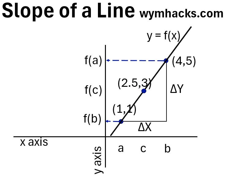
The slope using points a and b will be = Rise/Run
= Δy / Δx = (f(a) – f(b)) / (b-a)
= (5-1)/(4-1) = 4/3 = 1.33
Lines by definition have the same slope , so we’ll get the same slope for any other pair of points.
If we use points c and b
= (3-1)/(2.5-1) = 1.33
= (5-3)/(4-2.5) = 1.33
What if we wanted to find the slope of a curve?
Slope of a Curve
Consider the curve in the graph below.
Graph_Slope of a Curve
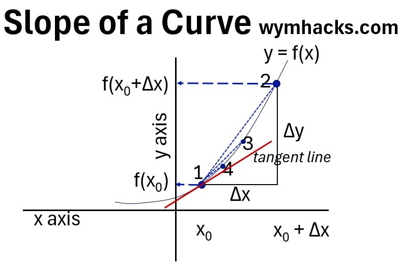
The Curve at each point has a different slope. So, What is the slope at point 1?
We still need two points to compute a slope so let’s choose Points 1 and 2 (see graph above).
- Slope 1 to 2 = Rise/Run = ∆y / ∆x
- Will give the slope of the Secant Line 12 (the dotted line between the two points in the graph)
This slope will not be very accurate.
We could compute the slope of Secant Line 13. It’ll be better but will still be off.
We could improve on this and compute the slope of Secant Line 14.
Ideally, if we could make the distance between the x points , ∆x, infinitely small, we would get the true slope at point 1.
We call this the slope of the tangent line at point 1 or the derivative of y = f(x) evaluated at point 1.
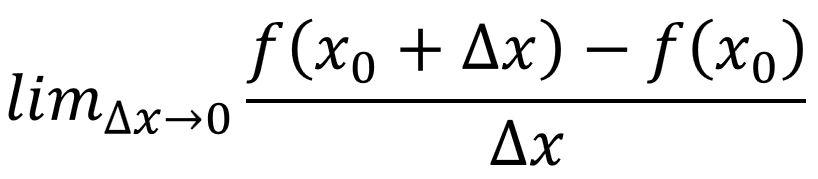
The general formula for a derivative states that
- as the limit of the difference in x values goes to zero,
- the slope will be equal to the (change in f(x))/(change in x).
or
We can notate the derivative in a few ways:
- Derivative of f(x)
- f prime x or f'(x) ; Lagrange Notation
- df(x)/dx = dy/dx; Leibniz Notation
- slope of tangent line at x
For a curve, each point has a unique tangent line with a unique slope (a unique derivative).
Check out these two nice introductory videos on the derivative:
Derivative Rules
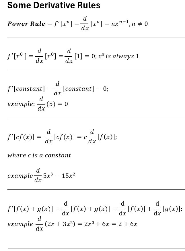
I’ve listed some of the main calculus derivative rules below.
Use Khanacademy.org’s excellent videos to learn more about these.
The primary rule for derivatives is the Power Rule and is defined as follows:
Power Rule: d/dx(xn) = nxn-1 where n cannot be zero.
- Example 1: the derivative of 3x3 is 3*3x2 = 9x2
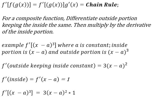
Another important one is the Chain Rule.
Product Rule: d/dx(uv) = (du/dx)v + u(dv/dx)
- Example 2: d/dx[(x+3)(x4)] = (1)(x4) + (x+3)(4x4) = 5x4 + 12x4
Chain Rule: fʹ[ f (g(x)) ] = fʹ(g(x)) gʹ(x)
- note that we used Lagrange Notation i.e. f prime = fʹ = derivative of f
- fʹ[ f (g(x)) ] = fʹ (outside[ ] keeping inside constant “times” fʹ inside ( )
- Example 3: fʹ (x2-a)3 = 3(x2-a)2(2x)…assuming a is a constant.
Table_Some Derivative Rules
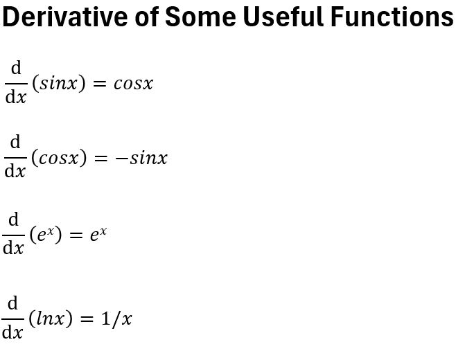
Derivatives of Some Useful Functions
We’ll also run into some functions we’ll need to take the derivatives of.
These are equalities that you would basically have to memorize if you were taking a calculus class.
Derivatives of sin(x) ,cos(x) , tan(x), cot(x), sec(x), csc(x)
- d/dx(sinx) = cosx
- d/dx(cosx) = -sinx
- !! These derivatives are only true if x is in units of Radians i.e. not degrees. (due to the limit assumptions made in the derivations).
Note that that the derivatives of the co-functions (cosine, cosecant, cotangent) are negative.
Example 4: Let x(t) = Acos(ωt + Φ) where A,ω, and Φ are constant
- dx/dt = dx/du * du/dt ; chain rule
- let u = ωt + Φ
- d(Acos(ωt + Φ))/dt = dx/du * du/dt = -Asin(( ωt + Φ)) * ω = -Aωsin(ωt + Φ)
Derivative of 𝑒ˣ
- d/dx(ex) = ex
- You can learn more at my blog on e (Euler’s Number) and ex
Derivative of ln(x)
- d/dx(lnx) = 1/x