Definitions
Let’s review some foundational definitions.
Rn
Rn represents the n-dimensional real coordinate space.
It is the set of all possible ordered lists (or tuples) of n real numbers.
Examples:
- the real line R1 (i.e. x line)
- the real coordinate plane R2 (i.e. xy plane) , and
- the real coordinate three-dimensional space R3 (i.e. xyz space) .
Scalar
Scalars are quantities with magnitude only.
A scalar is just a number.
Scalar examples in science are:
- mass, distance, speed, volume, temperature, energy
Vector
Vectors are quantities with magnitude and direction.
- position vectors (e.g. x̄ or x ; shown typically as a letter or other symbol with a line or arrow above it; or as bolded text)
- displacement vectors (Δx or Δx̄ )
- velocity, acceleration, force, etc.
See my post on vector math for more information and rules regarding vectors.
Function
A mathematical function is a rule that assigns to each input value (from a set called the domain) exactly one output value (from a set called the range).
- input → function → output
- Domain: This is the set of all possible input values that the function can accept.
- Range: This is the set of all output values that the function can produce.
- Unique Output: For every input in the domain, there must be only one corresponding output in the range.
- The equation for a circle, e.g. x2 + y2 = 4, is not a function
- If drawing a vertical line through the graph intersects the graph twice, then the related equation is not a function
Scalar Function
A scalar function, often written as f(x,y,z), takes one or more scalar inputs and produces a single scalar output. The output has magnitude but no direction.
Vector Function (Vector Valued Function)
You don’t need to know this for this post but I’m throwing it in for completeness.
A vector-valued function is a function
- whose input is a real parameter t
- and whose output is a vector that depends on t .
The graph of a vector-valued function is the set of all terminal points of the output vectors with their initial points at the origin.
Graph: (2D example) Vector Valued Functions Map Vectors to Curves
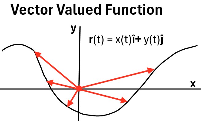
The î and ĵ are unit vectors (see my vectors post).
You can watch these two nice introductory videos on vector-valued functions.
- Vector-valued functions intro – Khanacademy
- Vectors, Vector Fields, and Gradients | Multivariable Calculus (time 5:22)
Field
In the sciences, a field represents a region of space where a physical quantity or mathematical value is assigned to each point.
- A field is a function that assigns a value (scalar or vector) to each point in a space.
- In physics, fields describe forces and influences extending through space and time, like gravity or electromagnetism.
Scalar Field (Scalar Field Function)
When the domain of a scalar function is a region in space (e.g., 2D or 3D physical space, or a surface), the scalar function effectively defines a scalar field.
A scalar field function is a type of scalar function that assigns a single scalar value to every point in a space,
Essentially, a scalar field is a specific application of a scalar function where the domain is a spatial region.
A generalized scalar field function, F, in three-dimensional space can be written as:
f(x,y,z)=C
where:
- x, y, and z are the coordinates of a point in space.
- C is a scalar value (a single number) assigned to that point.
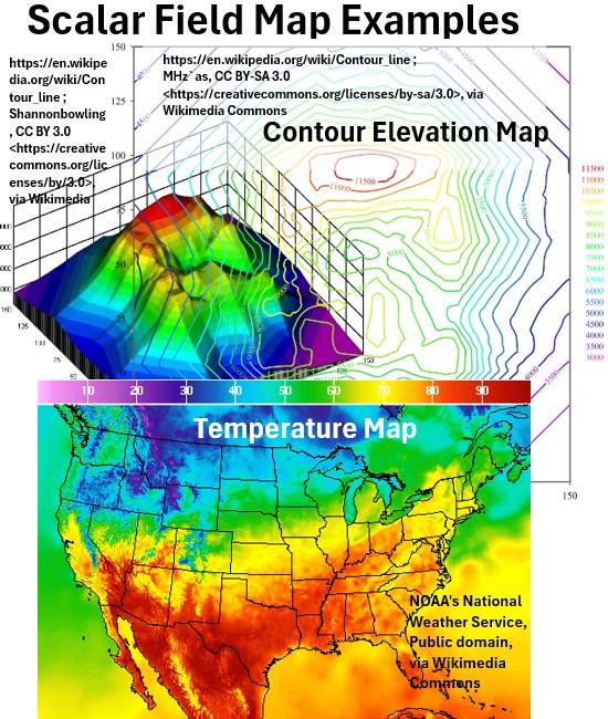
For example, a scalar field could represent
- the temperature at every point in a room, where
- the function f(x,y,z) gives a single temperature value at a specific location.
Other examples of Scalar Fields:
- Elevation contour map
- Pressure distribution
- Density (mass/volume) distribution
Vector Field (Vector Field Function)
A vector field function maps points in an n-dimensional space to vectors in that same n-dimensional space. e.g. 2D to 2D
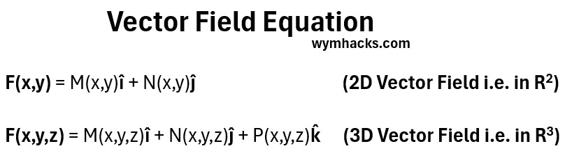
A generalized vector field function, F, in three-dimensional space can be written as:
F(x,y,z)=M(x,y,z)î + N(x,y,z)ĵ + P(x,y,z)k̂
where:
- x, y, and z are the coordinates of a point in space.
- î, ĵ , k̂ are the standard unit vectors along the x, y, and z axes.
- M, N, and P are scalar-valued functions that describe the components of the vector at each point.
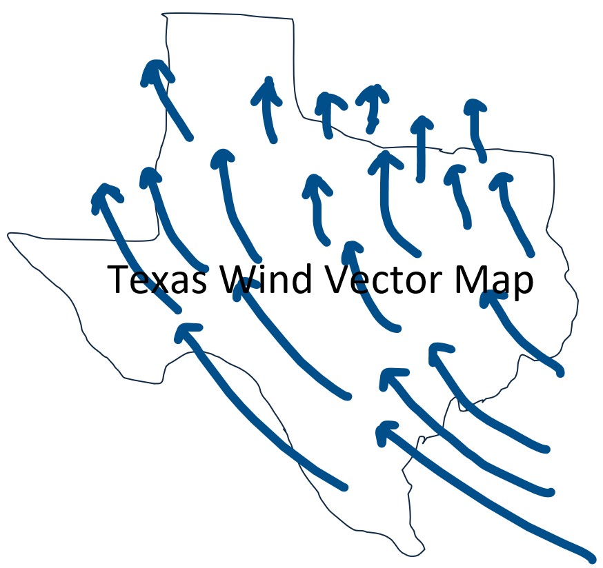
For example, a vector field could represent the velocity of wind at every point over Texas,
- where M, N, and P would describe the x, y, and z components of the air’s velocity at that location.
In 2D, we would only have the x,y space and the î and ĵ unit vectors, and so the vector equation becomes:
F(x,y)=M(x,y)î + N(x,y)ĵ
Vector Field Example: Wind Velocity and Direction Weather Map
Vector Field Example: Electric Field From A Single Positive Charge (Source: PHET)
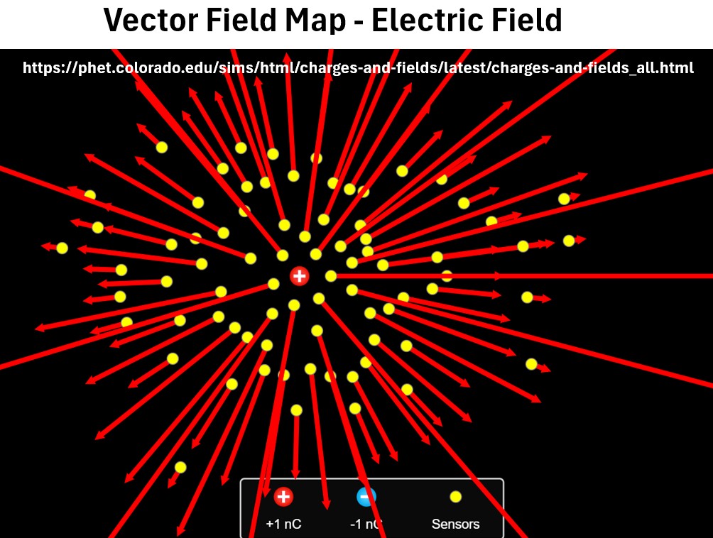
In the electric field map above, notice how the vectors all point out symmetrically and radially from the source charge.
In the next section we’ll learn how to graph some basic vector fields.
Graphing Vector Fields
- take various domain input (x,y) points and
- generate vectors xî + yĵ for each one.
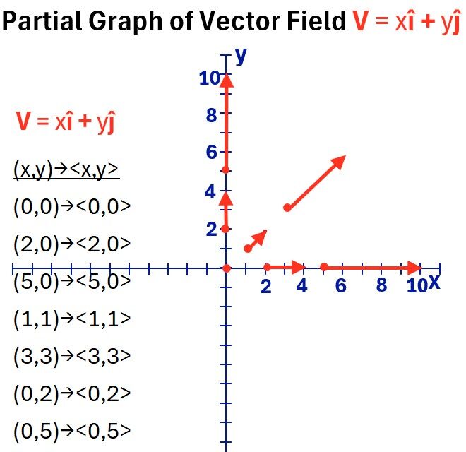
For each input (x,y) we’ll produce an output (xî + yĵ) allowing us to draw the vector.
(0,0)→<0,0>
- From point (0,0) move 0 to the right (+x), and o up (+y)
- this is just the point at (0,0)
- So plot the point (0,0)
(2,0)→<2,0>
- Starting at (2,0) go 2 to the right and 0 up
- Draw the vector line from (2,0) to (4,0)
(5,0)→<5,0>
- Starting at (5,0) go 5 to the right and 0 up
- Draw the vector line from (5,0) to (10,0)
(1,1)→<1,1>
- Starting at (1,1) go 1 to the right and 1 up
- Draw the vector line from (1,1) to (2,2)
(3,3)→<3,3>
- Starting at (3,3) go 3 to the right and 3 up
- Draw the vector line from (3,3) to (6,6)
(0,2)→<0,2>
- Starting at (0,2) go 0 to the right and 2 up
- Draw the vector line from (0,2) to (0,4)
(0,5)→<0,5>
- Starting at (0,5) go 0 to the right and 5 up
- Draw the vector line from (0,5) to (0,10)
etc..
You get the idea.
We can view a pattern emerging in the vectors we’ve drawn.
The vectors are radiating outwards from the origin and get larger as they move away.
Graph_1: Partial Graph of Vector Field Function V(x,y) = xî + yĵ
I found a cool on line plotter which I’ve used to generate a more complete vector field for our example (see Graph 2 below).
Graph_2: Diverging Vector Field Function V = V(x,y) = xî + yĵ
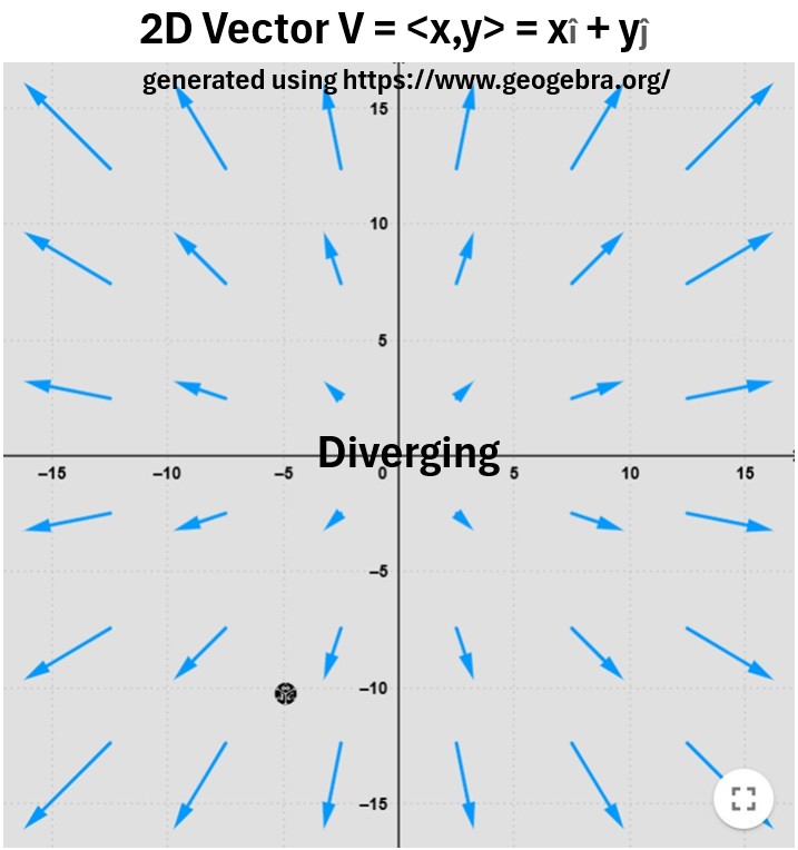
Graph 2 is an example of vectors radiating (or diverging) and increasing from a central source.
I generated a few more in Graphs 3 through 7.
Graph_3: Converging Vector Field Function V = -xî – yĵ
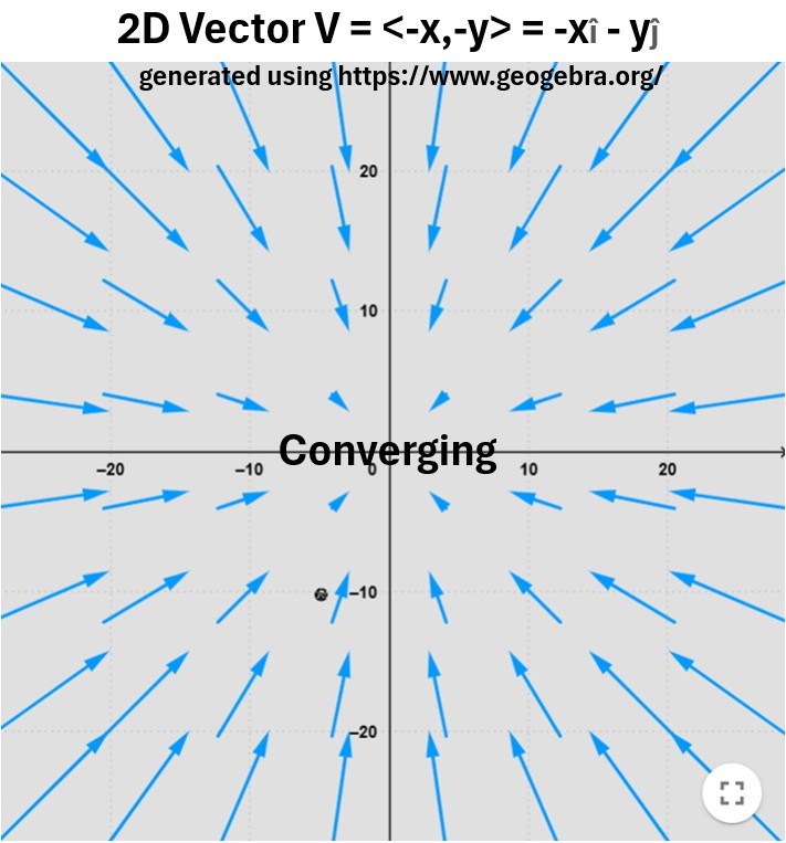
Graph 3 shows vectors converging and shrinking towards a center point (or sink).
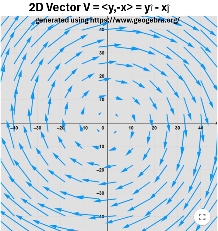
Graph_4: Spiral Vector Field Function V = yî – xĵ
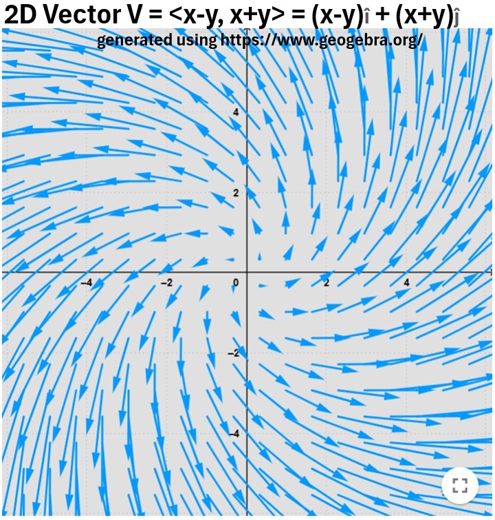
Graph_5: Spiraling Vector Field Function V = (x-y)î + (x+y)ĵ
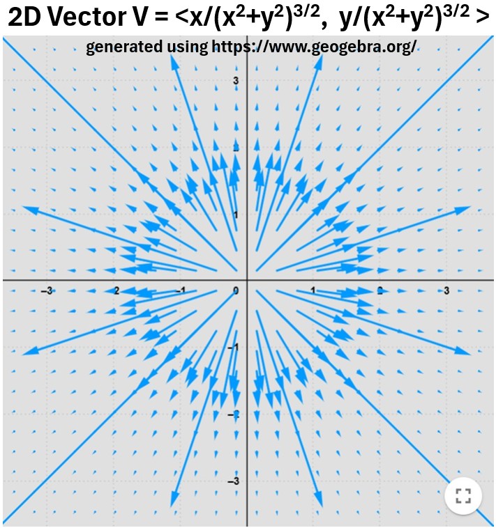
In Graphs 6 and 7 below I’ve drawn the 2D and 3D versions of a generalized electric field due to a point charge.
You can see it diverges outwards from its electric charge source, but unlike Graph 2 the vector magnitudes decrease as they move away from the origin.
This makes sense since Electric Field strength gets weaker as the point of interest moves away from the source charge.
Graph_6: Electric Charge Field Function
V= (x/(x2+y2)3/2)î +(y/(x2+y2)3/2)ĵ
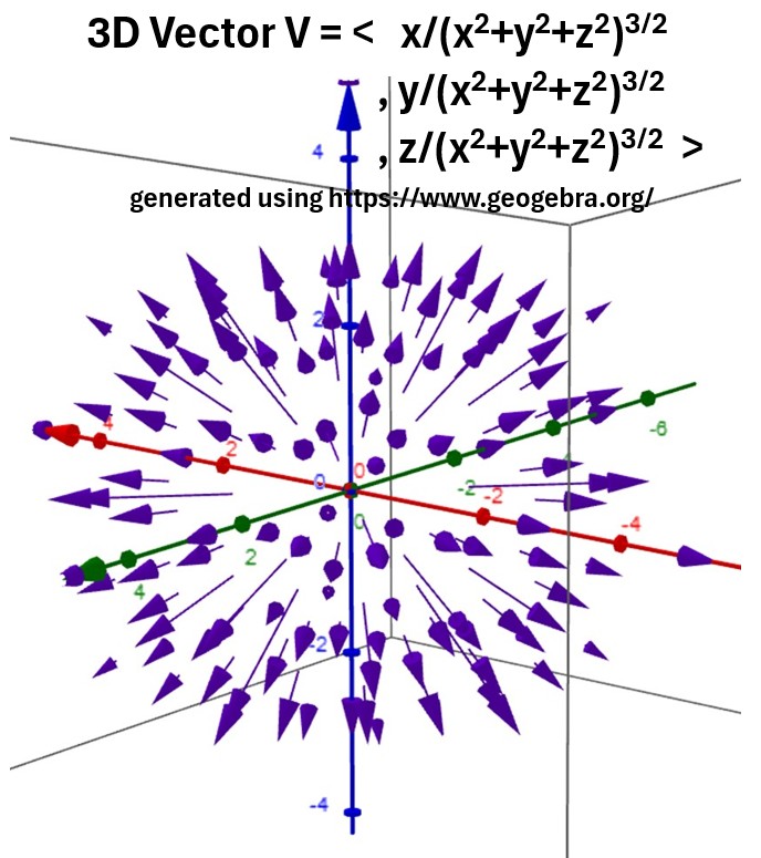
Everything we’ve talked about works in 3d space too.
So, in Graph 7, we see that the Electric field radiates outwards from the source charge in all directions.
Graph_7: 3D Electric Charge Field
V= (x/(x2+y2+z2)3/2)î +(y/(x2+y2+z2)3/2)ĵ+(z/(x2+y2+z2)3/2) k̂
Differentiation Basics
Derivative
The derivative of a function
- measures the instantaneous rate of change of that function with respect to one of its variables.
- It represents the slope of the tangent line to the function’s graph at a specific point.
For a function f(x), its derivative, often denoted as f′(x) or df/dx, tells us how sensitive the function is to small changes in x.
Graph: Derivative (Slope of a Curve)
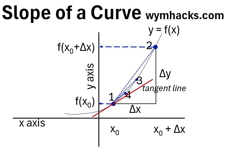
For a function , its derivative, denoted as , is defined as:
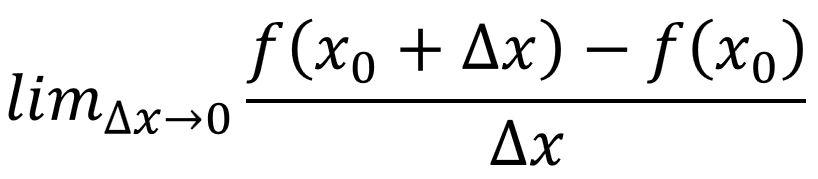
- the second point gets infinitesimally close to the first, and
- the secant line’s slope becomes the instantaneous slope of the tangent line at point .
Partial Derivative
A partial derivative is a derivative of a function with multiple variables, where you treat all other variables as constants.
- For a function f(x,y), the partial derivative with respect to x, denoted as ∂f/∂x , measures
- how f changes as you change only x and hold y constant.
- Similarly, ∂f/∂y measures the rate of change with respect to y, with x held constant.
Importance
Derivatives are fundamental to modern science and technology as they measure the rate of change.
- The derivative is essential for understanding the dynamics of systems that change over time,
- while the partial derivative is crucial for modeling complex systems where a result depends on multiple independent factors.
This ability to describe how a system changes is crucial for modeling and predicting real-world phenomena.
They are used to
- find maximum and minimum values of functions,
- optimize processes in engineering and economics,
- and describe physical phenomena such as velocity, acceleration, and the flow of heat or fluids.
One of many real world application of differentials is in electromagnetism.
- The rules which govern how electric and magnetic fields behave and interact are expressed using differential equations. (Maxwell’s Equations).
- These equations use derivatives to describe how these fields change in space and time.
- They are the basis for technologies like radio, television, and wireless communication.
See Appendix I for examples of where derivatives are applied.
The Gradient Operator (scalar → vector)
![]()
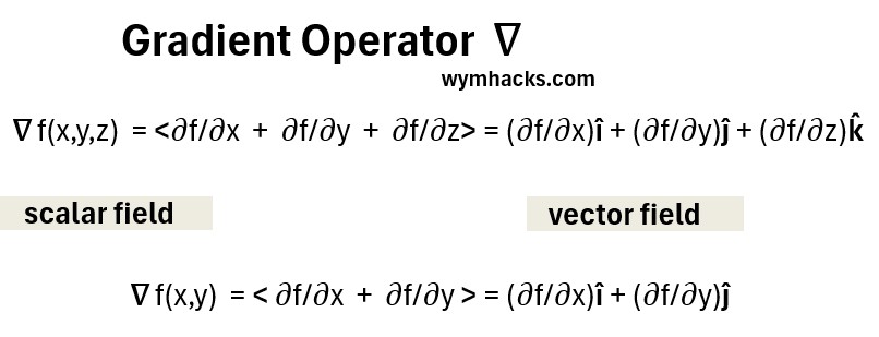
The gradient operator, denoted by (nabla or del), takes a scalar-valued function of several variables and produces a vector.
- The gradient operator is exclusively applied to a scalar field.
- The result of this operation is always a vector field
The resultant vector, known as the gradient,
- points in the direction of the steepest increase of the function.
- Its magnitude represents the rate of that steepest increase.
Lets do the math to clarify this by first recalling that the two common vector notation formats are:
- the bracket format < x,y,z > and
- the unit vector format xî + xĵ + xk̂
- Note that they represent the exact same thing.
So, for a scalar function , the gradient of f(x,y,z) or grad f or is calculated by taking the partial derivative of the function with respect to each variable and forming a vector from these derivatives:
∇ f(x,y,z) = <∂f/∂x, ∂f/∂y, ∂f/∂z> = (∂f/∂x)î + (∂f/∂y)ĵ + (∂f/∂z)k̂
Gradient Analogy
- Think of the gradient like being on a hill represented by a function.
- The gradient at your position on the hill is a vector that points in the direction you should walk to go uphill as quickly as possible,
- and the length of that vector tells you how steep the hill is in that direction.
- The gradient vector is also always perpendicular to the level curves (or surfaces) of the function.
Gradient Example: f(x,y) = .5(x2 + y2)]
- f(x,y) = .5(x2 + y)2
- x2 + .5y2x2 + .5y2
- We just took the derivative with respect to x and y (using the power rule )
- shown on the left and also
- on the right as the x,y “floor” in the 3D space that holds the surface graph of the paraboloid.
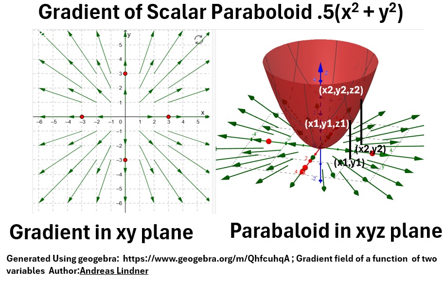
Note the following observations on the graphs above:
- The output of the gradient operator on a 2D scalar function, is a vector field in the xy plane (the graph above on the left).
- We’ve seen this field before. We drew it in a previous section:
- Its a diverging field from a source at (0,0).
- If we pick a point on the x,y plane we can compute the z component by plugging those values into the function .5(x2 + y)2.
- This will map out a paraboloid in the x,y,z dimension.
- The gradient at that z position on the paraboloid is a vector that points in the direction of steepest ascent,
- and the length of that vector tells you how steep the paraboloid is in that direction.
- As the vectors move outward they indicate a steeper paraboloid region as indicated by their increasing length.
Ok, that’s pretty cool.
Gradient Properties
The Directional Derivative
So, the gradient is a vector that points in the direction of the steepest ascent and tells us the rate of change in that direction.
But what if we’re not interested in the steepest direction?
What if we want to know the rate of change of our function in any arbitrary direction we choose?
We compute the Directional Derivative to know this.
It is the measure of how a function changes as you move in a specific, predetermined direction (any direction).
The Directional Derivative of a function f in the direction of a unit vector u is the dot product of the gradient of f and u.
Duf = ∇f⋅u
The equation takes the “steepest ascent” vector (the gradient, ∇f) and finds its component in your chosen direction (u) via the dot product.
This dot product essentially gives you the “projection” of the gradient onto your chosen direction, telling you how much the function is changing as you move along that path.
To gain a better understanding you probably need to understand this graph
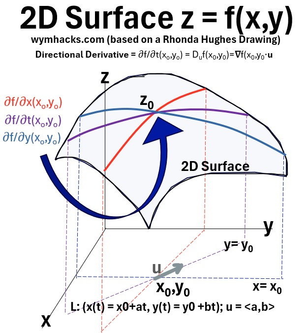
and watch these three videos:
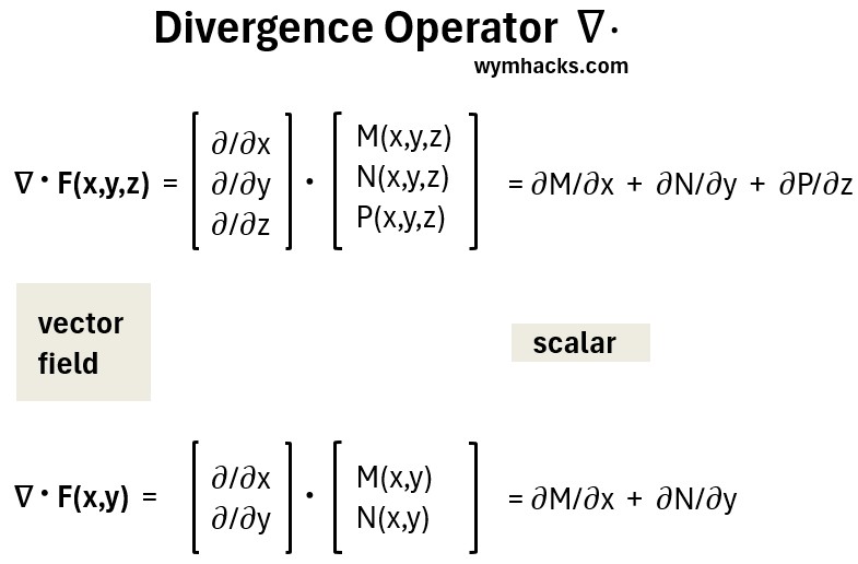
Divergence Operator (vector → scalar)
- The gradient operator (∇) is exclusively applied to a vector field and
- the result (the divergence) of this operation is always a scalar field
The Divergence is a scalar value that measures the “outflowing-ness” of a vector field at a specific point.
- Imagine the vector field as a fluid flow.
- The divergence at a point tells you if that point is a source (positive divergence, fluid is flowing out) or
- a sink (negative divergence, fluid is flowing in).
- If the divergence is zero, the fluid is neither expanding nor contracting at that point.
So let’s first define a vector field in 3D as F(x,y,z) where,
F(x,y,z) = M(x,y,z)î+N(x,y,z)ĵ+P(x,y,z)k̂
where:
- x, y, and z are the coordinates of a point in space.
- î, ĵ , k̂ are the standard unit vectors along the x, y, and z axes.
- M, N, and P are scalar-valued functions that describe the components of the vector at each point.
The Divergence of F is the dot product of the gradient operator and a vector field F:
Divergence F = div F = divF = ∇•F = ∂M/∂x + ∂N/∂y +∂P/∂z
The divergence shows how much F is sourcing in or syncing out.
Divergence Properties
Example 1
Consider the vector field F(x,y) = xî + yĵ
∂M/∂x + ∂N/∂y = 2
So divF = 2 . It is a positive value, which means the vector field is sourcing out (radiating out from center).
And that’s what we see when we plot the vector field xî + yĵ
Example 2
Consider the vector field F(x,y) = -xî + –yĵ
∂M/∂x + ∂N/∂y = -2
So divF = -2 . It is a negative value, which means the vector field is syncing in (converging) to center.
And that’s what we see when we plot the vector field -xî + –yĵ
Example 3
Consider the vector field F(x,y) = yî – xĵ
∂M/∂x + ∂N/∂y = 1-1 = 0
So divF = 0 which means the vector field is not syncing or sourcing (its rotating).
And that’s what we see when we plot the vector field yî + –xĵ
The Laplacian (scalar → scalar)
The divergence of the gradient of a function is a special differential operator called the Laplacian (luh-PLAH-shun or luh-PLAY-shun).
The Laplacian is a scalar operator that takes a scalar function (or “scalar field”) and returns a new scalar function.
This operation is written as ∇•(∇f), which is often simplified to ∇2f or Δf.
Step 1: ∇f
We’ve seen that the gradient of a scalar function creates a vector:
grad f = ∇ f(x,y,z) = <f/x, f/y, f/z>
Step 2: ∇•(∇f)
Now, take the divergence of this resulting vector field to produce a scalar:
∇•(∇f) = /x(f/x)+/y(f/y)+/z(f/y)
This simplifies to the sum of the second-order partial derivatives, which is the definition of the Laplacian:
∇2f = ∂2f/∂x2 + ∂2f/∂y2 + ∂2f/∂z2
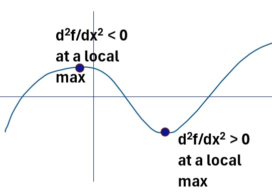
Physical Meaning
The Laplacian measures how a function’s value at a point deviates from the average of its neighbors.
It’s a measure of concavity, the rate of change of slope as you move away from the starting point.
- A positive Laplacian indicates that the point is a “source” or local minimum, while
- a negative Laplacian indicates a “sink” or local maximum.
- A Laplacian of zero means the function is harmonic at that point, indicating a smooth, stable, or equilibrium state.
Consider the Laplacian of a function f(x,y): ∇•(∇f)
- The 2D function can be visualized as a 2D surface situated in 3D (with possible hills and valleys).
- The value of the function, f(x,y), tells you the height of the surface at each (x,y) point.
- ∇f will be the gradient of f which is a vector field in the (x,y) plane.
- The gradient, ∇f, tells you the direction and steepness of the slope at that point.
- The vectors point up the steepest parts of the hills or valleys on the function surface.
- The divergence of this vector field is the Laplacian: ∇•(∇f).
- The Laplacian, as a second derivative, is a measure of curvature.
- , the resulting value (the Laplacian) indicates the concavity of the surface at that point.
- It’s analogous to the concavity of a single variable function
- The Laplacian at a point says nothing about the value of the function at that point, but rather describes the behavior of the function in the infinitesimally small neighborhood around it
- It’s fundamentally a statement about how the function’s value changes as you move away from the point in all directions.
- The Laplacian is defined by the values of the function’s neighbors, not the point itself
Application in the Real World
The Laplacian, is widely used in various scientific fields like physics, engineering, and computer science.
- It appears in equations describing phenomena like heat transfer, wave propagation, and quantum mechanics.
- Its applications include solving partial differential equations, analyzing fluid flow, and smoothing surfaces in computer graphics.
Direction of an Axis of Rotation
The curl mathematical operator produces information on how things rotate.
Before I talk about it, we need to understand a convention that allows us to remove any ambiguity from describing rotation.
Look at the picture below where I show 2 persons that have two different perspectives when they view the circular rotation of an object.
- One person sees the motion as clockwise, while
- the other person see the same motion as counterclockwise.
Picture: Rotational Vector – Right Hand Rule
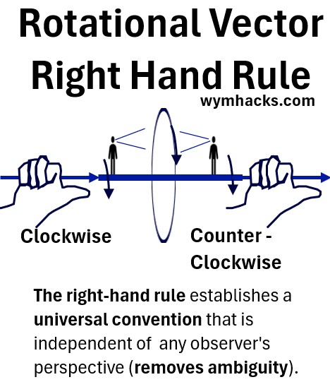
To remove the ambiguity that is cased by the position of the viewer, we apply the Right Hand Rule for rotation.
Right Hand Rule for Rotation
- Take your right hand and
- Curl your fingers in the direction of rotation.
- Your thumb then points in the direction of the curl vector.
- This vector indicates the axis of rotation
See the picture below where I show a sphere rotating around its axis.
Picture: Angular Velocity and Right Hand Rule
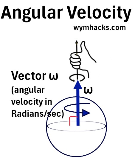
The angular velocity ω (omega in Radians/second typically) is the rate of rotation around the axis of rotation and L = Iω where
- L = Angular Momentum (a vector)
- ω = Angular Velocity (a vector)
- I = Rotational Inertia of the Object ( a function of mass and distance to center)
Applying the Right Hand Rule to the picture above,
- the rotational axis, which is the direction of both vectors ω and L, is pointing upwards.
- If the rotation was clockwise, the vector would be pointing downwards.
This vector is perpendicular to the plane of rotation.
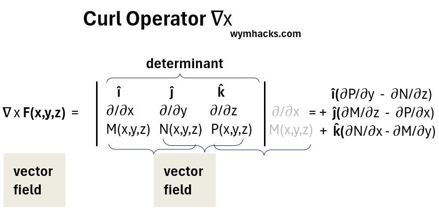
Curl Operator (vector → vector)
Curl Definition
The curl measures the rotation (or curl) of a 3D vector field, and the result is another 3D vector field.
Given the general equation for a 3D vector field,
F(x,y,z) = M(x,y,z)î + N(x,y,z)ĵ + P(x,y,z)k̂ (3D Vector Field i.e. in R3)
where:
- x, y, and z are the coordinates of a point in space.
- î, ĵ , k̂ are the standard unit vectors along the x, y, and z axes.
- M, N, and P are scalar-valued functions that describe the components of the vector at each point.
The curl of F(x,y,z) is defined as the cross product of the del (nabla) operator and the vector field.
= î(P/y – N/z)
+ ĵ(M/z – P/x)
+ k̂(N/x – M/y)
note: Technically, The del operator is NOT A VECTOR, but by treating it as one we can use the cross product methodology to compute the curl.
Picture: Curl Operator
Example 1: Computing the Curl
Let F(x,y,z) = M(x,y,z)î + N(x,y,z)ĵ + P(x,y,z)k̂ = (xy)î + (-sin z)ĵ + (1)k̂
= î(P/y – N/z)
+ ĵ(M/z – P/x)
+ k̂(N/x – M/y)
= î(1/y – (-sin z)/z))
+ ĵ((xy)/z – /x))
+ k̂((-sin z)/x – (xy)/y))
= î(cos z) + ĵ(0) – k̂(x)
So, we took the curl of a vector field, and our result is another vector field: the curl vector field.
We said the curl is an indicator of rotation but what does this look like on a graph?
Let’s look at Example 2 to understand this.
Example 2:
Let’s take the curl of a vector field in which the z component is zero.
Let F(x,y,z) = M(x,y,z)î + N(x,y,z)ĵ + (0)k̂ =
= î(P/y – N/z)
+ ĵ(M/z – P/x)
+ k̂(N/x – M/y)
In this case P is zero and all the partials with respect to z are zero so
= k̂(N/x – M/y)
= a curl vector field that is only pointing in the z direction, which is therefore perpendicular to the xy plane.
Example 3:
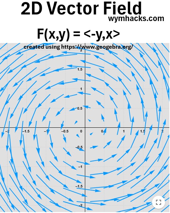
Let’s repeat example two on the specific vector field function: F(x,y,z) = <-y,x,0>
This is the 3D analogue of the rotating 2D vector field F(x,y) = <-y,x> which is shown in the graph below.
Picture: F(x,y) = <-y,x> Vector Field
Lets convert this 2D function graph into its analogous 3D function graph:
- So we want to convert the graph of F(x,y) = <-y,x> into
- the graph for F(x,y,z) = <-y,x,0>.
- Imagine that you take an infinite number of vector fields like the one above and stack them up in the xy plane direction in 3D space.
Then, you get the graph below.
Picture: Graph of F(x,y,z) = <-y,x,0>
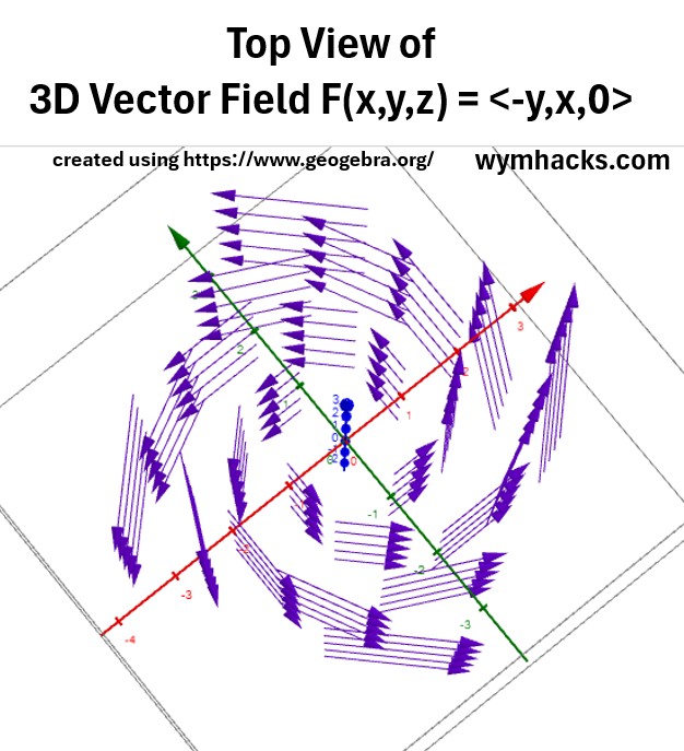
So, you get it, you get a graph of an infinite stack of vector fields in the XY plane.
Now lets take the curl of F(x,y,z):
= k̂(N/x – M/y)
= (1 + 1)k̂ = 2k̂
So the result is a Curl vector field with vectors of magnitude 2 pointing in the z direction.
Let’s incorporate these Curl vector fields onto our 3D vector field graph.
Picture: Curl of Vector Field
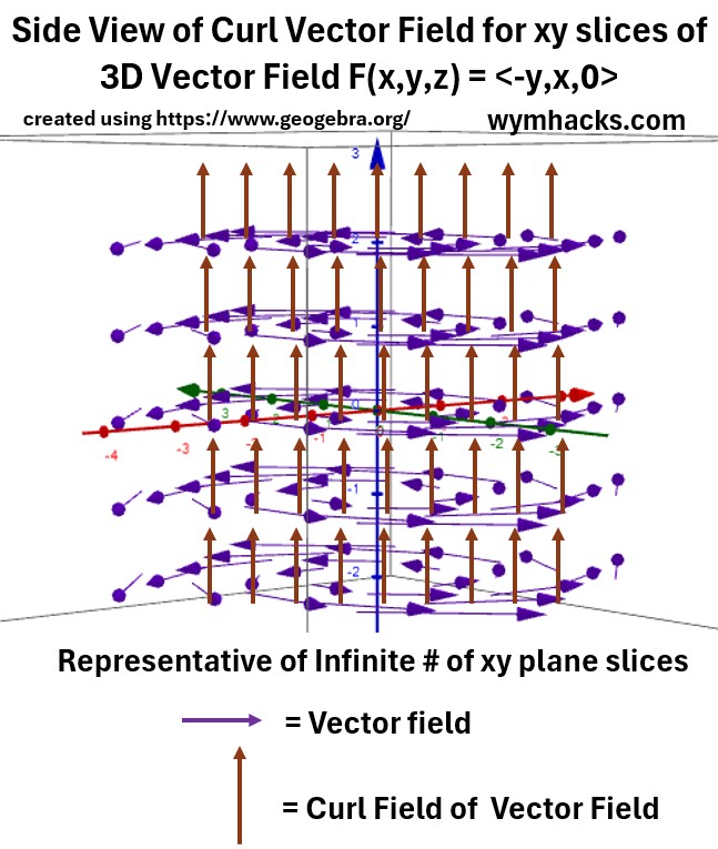
Voila.
Description of Graph Above
- An infinite number of xy planes stacked up the z axis.
- Each plane contains the same flow vector fields, embedded in the xy plane.
- Each plane has an associated curl vector field.
- The curl vector field has vectors emanating from the xy plane and pointing vertically upwards
- with a magnitude of 2 (identically for each plane).
- Using the Right Hand Rule and given the rotation direction (counterclockwise),
- the curl vector will point up,
- perpendicular to the rotating xy plane.
- The curl is a positive, another indication that the rotation is counterclockwise.
It Can Get Very Complicated
We simplified the 3D function graph above by providing a simple vector field with a zero z (k) component.
You can imagine how these can get a lot more complicated with no easy visual to help us make sense of the vector fields and their curl fields.
You really have to think about each singular curl vector resulting from each singular location in 3D space.
See the picture below.
Picture – Fluid Curl Vectors
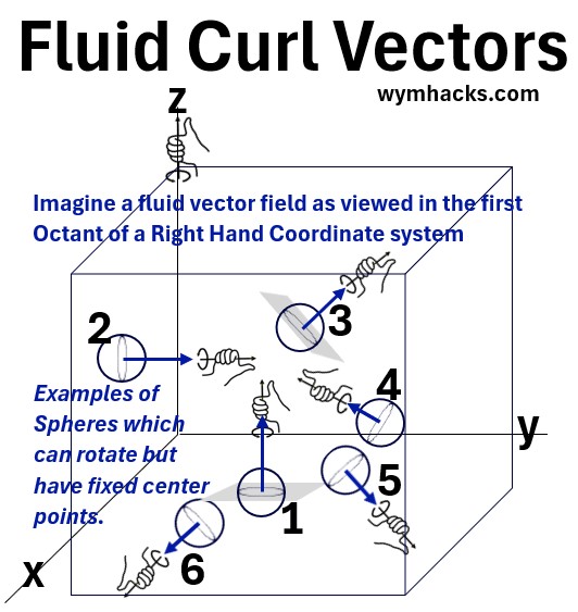
Imagine all the points in 3D space being represented as infinitesimally small spheres.
- Each sphere is fixed at its center but can otherwise rotate in any direction.
- Each sphere will eventually line up along its axis of rotation.
- This will be perpendicular to the plane of rotation.
- The Right Hand Rule will dictate which way the vector points.
- The Vector lengths can change indicating differing rates of rotation.
The 2D Analog of a Curl
Let’s look at example 2 again:
Let F(x,y,z) = M(x,y,z)î + N(x,y,z)ĵ + (0)k̂.
= î(P/y – N/z)
+ ĵ(M/z – P/x)
+ k̂(N/x – M/y)
P is zero and all the partials with respect to z are zero so
= k̂(N/x – M/y)
We can define a scalar curl or 2D curl as
curl F(x,y)=∂N/∂x−∂M/∂y
This scalar value
- represents the magnitude of the rotation and
- it’s sign indicates the direction of the rotation
- Positive if counterclockwise and
- Negative if clockwise
- The sign also indicates the direction of the axis of rotation
- Pointing up if counterclockwise and
- Pointing down if clockwise
- This scalar value is essentially the -component of the 3D curl vector, which is why it can fully describe the rotation for a 2D field.
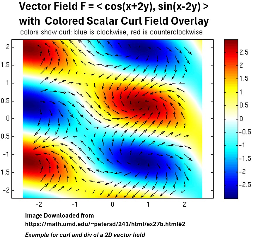
For a 2D vector field the curl will be a scalar vector field.
This can be shown on an xy graph as a colored or contoured overlay.
See the great example shown in the graph below.
Graph: Example of 2D Vector Field with Colored Scalar Curl Field Overlay
Properties of the Curl
The Curl of the Gradient of a scalar function f(x,y,z) is a <0,0,0> vector field
The Divergence of the Curl of a vector field F is always zero
- •(
The vector identity for the Curl of a Curl of a vector field F is:
- ∇×(∇×F) = ∇(∇⋅F)−∇2F where
- ∇(∇⋅F) is the gradient of the divergence of A.
- The divergence (∇⋅A) is a scalar function,
- and the gradient (∇) of that scalar function produces a vector field.
- This term represents the “source” or “flow” part of the vector field.
- ∇2F is the vector Laplacian of F.
- It’s the Laplacian operator applied to each component of the vector field,
- resulting in another vector field.
- It represents the “diffusion” or “spread” part of the vector field.
- The derivation of this is quite complicated so I am not including it in this post.
- This identify is used to derive the wave equation from Maxwell’s electromagnetic equations.