Integration Definition and Rules

Menu (linked Index)

Integration Rules

Last Update: July 1, 2025

Introduction
Integral Definition
Integral Notation
Integration: Basic Formulas
Beyond basic integration

Introduction

Finding the area under a curve in physics is very useful.

For example, the work done on an object that is displaced a distance d is computed as W = force x distance.

This can be plotted to produce a graph perhaps similar to the one shown below in the next section.

The area under the force curve would then represent the work.

The process of computing this area is called integration.

In this post I introduce the definition of an integral and provide some of the basic math involved in taking integrals.

Return to Menu

The Concept of Integration

Integration is the process of finding the total or accumulation of a quantity.

An integral is the mathematical result of this process, representing either:

The antiderivative: A function whose derivative is the original function (indefinite integral, often written as $\int f (x) d x$ ).
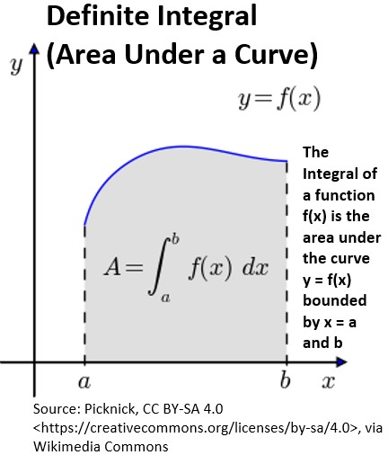
The net area under a curve: The total value accumulated between specific points a and b (definite integral, written as $\int a b f (x) d x )$

$<img decoding="async" class="alignnone size-full wp-image-30380" src="https://wymhacks.com/wp-content/uploads/2025/07/2025.04.21-definite-integral-area-under-curve-wiki-chart-.jpg" alt="" width="432" height="506" />$

Integration is essentially the reverse process of differentiation.

Return to Menu

Notation

Indefinite Integral (Antiderivative): $\int f (x) d x = F (x) + C$

$\int$ : The integral symbol.
$f (x)$ : The integrand (the function you want to integrate).
$d x$ : The differential, indicating that you’re integrating with respect to the variable $x$ .
$F (x)$ : The antiderivative of $f (x)$ (meaning $F^{'} (x) = f (x)$ ).
$C$ : The constant of integration.
- The derivative of any constant is zero, so when you reverse the process, you don’t know what constant was there originally.

Definite Integral (Area Under a Curve): $\int a b f (x) dx = F (b) - F (a)$

- $a$ : The lower limit of integration.
- $b$ : The upper limit of integration.
- This calculates the net area between the curve $f (x)$ and the x-axis from $x = a$ to $x = b$ .

Return to Menu

Basic Integration Formulas (Rules for Antiderivatives)

These are the fundamental “formulas” you’ll use most often.

For a definite integral (integrating within an upper and lower limit), the C in the formulas below disappear because they cancel out.

Power Rule (for $n \neq - 1$ )

$\intx n dx = x (n+1) /(n+1) + C$
Example: $\intx 3 dx = x (3+1) /(3+1) + C = x 4 /4 + C$
Example: $\int 1dx =$ $\intx 0 dx = x 1 /1 = x$

Power Rule (for $n = - 1$ )

$\int 1/x = \int x -1 d x = ln ∣ x ∣ + C$
$∣ x ∣ = absolute value of x$
Example: $\int 1 d t = ln ∣ t ∣ + C$

Constant Multiple Rule

$\int c f (x) d x = c \int f (x) d x$
Example: $\int 5 x 2 d x = 5 \int x 2 d x = 5 (x 3) + C = 5/3 + C$

Sum/Difference Rule

$\int [f (x) \pm g (x)] d x = \int f (x) d x \pm \int g (x) d x$
Example: $\int (x 2 - 3 x + 1) d x = \int x 2 d x - \int 3 x d x + \int 1 d x = x 3 - 3 x 2 + x + C$

Integral of a Constant

$\int c d x = c x + C$
Example: $\int 7 d x = 7 x + C$

Trigonometric Integrals

$\int cos (x) d x = sin (x) + C$
$\int sin (x) d x = - cos (x) + C$
$\intsec 2 (x) d x = tan (x) + C$
$\intcsc 2 (x) d x = - cot (x) + C$
$\int sec (x) tan (x) d x = sec (x) + C$
$\int csc (x) cot (x) d x = - csc (x) + C$

Exponential Integrals

$\inte x d x = e x + C$
$\inta x d x = a x /ln a + C$ (for $a > 0, a\neq 1$ )

Return to Menu

Integration Techniques Beyond Basic Formulas

When the function isn’t a simple form, various techniques can be used to find a solution.

For a particular problem, you can mostly likely find the complete solution by asking your preferred AI app (like Google Gemini for example).

I will list examples here when relevant to other blogs I have written:

Example 1: Take the integral of (V/L)sin(ωt)dt

∫(V/L)sin(ωt)dt

Pull out the constants

(V/L)∫sin(ωt)dt

Integrate sin(ωt) using substitution technique

This requires a $u$ -substitution, where

$u = \omega t$ ωt and
$du = \omega dt$
$dt = \frac{1}{\omega} du$ .

(V/L)(1/ $dt = \frac{1}{\omega} du$ ∫sin(u)du

From the trig integrals we know that ∫sin(u) = -cos(u) so

(V/L)(1/ $dt = \frac{1}{\omega} du$ (u)) + Constant

Rearrange and substitute ωt for u

∫(V/L)sin(ωt)dt = -V/(Lω)(cos(ωt) + C

The term ω is typically the angular frequency in physics and engineering contexts (like AC circuits), while V/L is often a constant related to voltage and inductance.

Example 2: Placeholder

Example 3: Placeholder

Return to Menu

Disclaimer: The content of this article is intended for general informational and recreational purposes only and is not a substitute for professional “advice”. We are not responsible for your decisions and actions. Refer to our Disclaimer Page.

Cookie	Duration	Description
cookielawinfo-checkbox-analytics	11 months	This cookie is set by GDPR Cookie Consent plugin. The cookie is used to store the user consent for the cookies in the category "Analytics".
cookielawinfo-checkbox-functional	11 months	The cookie is set by GDPR cookie consent to record the user consent for the cookies in the category "Functional".
cookielawinfo-checkbox-necessary	11 months	This cookie is set by GDPR Cookie Consent plugin. The cookies is used to store the user consent for the cookies in the category "Necessary".
cookielawinfo-checkbox-others	11 months	This cookie is set by GDPR Cookie Consent plugin. The cookie is used to store the user consent for the cookies in the category "Other.
cookielawinfo-checkbox-performance	11 months	This cookie is set by GDPR Cookie Consent plugin. The cookie is used to store the user consent for the cookies in the category "Performance".
viewed_cookie_policy	11 months	The cookie is set by the GDPR Cookie Consent plugin and is used to store whether or not user has consented to the use of cookies. It does not store any personal data.

Menu (linked Index)

Introduction

The Concept of Integration

Integration is the process of finding the total or accumulation of a quantity.

Notation

Indefinite Integral (Antiderivative): ∫f(x) dx=F(x)+C

Definite Integral (Area Under a Curve): ∫ab f(x)dx = F(b)−F(a)

Basic Integration Formulas (Rules for Antiderivatives)

Power Rule (for n ≠−1)

Power Rule (for n=−1)

Constant Multiple Rule

Sum/Difference Rule

Integral of a Constant

Trigonometric Integrals

Exponential Integrals

Integration Techniques Beyond Basic Formulas

Example 1: Take the integral of (V/L)sin(ωt)dt

Pull out the constants

Integrate sin(ωt) using substitution technique

Example 2: Placeholder

Example 3: Placeholder

Leave a Comment Cancel Reply

Indefinite Integral (Antiderivative): $\int f (x) d x = F (x) + C$

Definite Integral (Area Under a Curve): $\int a b f (x) dx = F (b) - F (a)$

Power Rule (for $n \neq - 1$ )

Power Rule (for $n = - 1$ )