
Fossil Fuels Defined
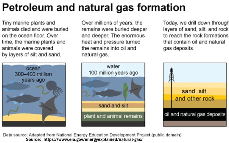
According to the US Department of Energy , “Fossil energy sources, including oil, coal and natural gas, are non-renewable resources that formed when prehistoric plants and animals died and were gradually buried by layers of rock.
Over millions of years, different types of fossil fuels formed — depending on what combination of organic matter was present, how long it was buried and what temperature and pressure conditions existed as time passed.”
Schematic: EIA.Gov Petroleum and Natural Gas Formation
Oil is also called Petroleum.
Several different kinds of fuels can be generated from refining Petroleum. For example:
- Transportation fuels like Gasoline, Diesel, and Jet Fuel
- Heating and industrial fuels like Heating Oil (Fuel Oil), Liquefied Petroleum Gas (LPG = primarily butane and propane), and Refinery Fuel Gas (Mostly Methane, Hydrogen, C2 and C3 hydrocarbons
Global and USA Energy Usage By Source
A vast majority of our energy usage is sourced by fossil fuels (about 81% globally and 83% for the USA).
Consider the two charts below for energy usage by source (globally and for the USA).
note: Primary Energy means before it gets converted to electricity or other forms of fuel
Chart: Global Primary Energy Use by Source 2025
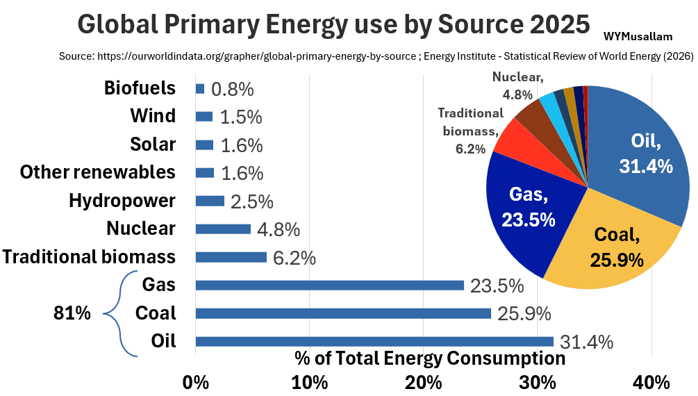
Chart: Global Primary Energy Use by Source 2025
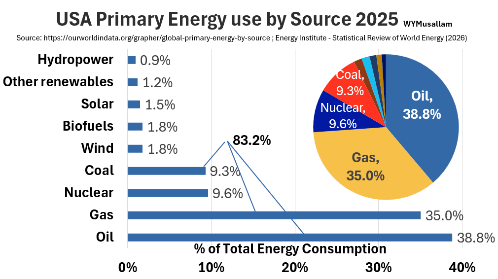
Without Fossil Fuels, Modern, Civilized Living Would Not Be Possible
- This is certainly absolutely true today.
- Renewables are “cleaner fuels but not always available
- Nuclear is the cleanest but comes at great cost and risk (perceived and real)
So globally, the chart above shows that 83.2% of global energy usage comes from Fossil Fuels.
- Be aware that the energy used is in reference to the energy content of the item (oil or gas).
- For fossil fuel, roughly 90% will be combusted (burned) to provide heat and power for all sorts of commercial and private applications.
- So about 83.2% x 90% = 75% of our energy comes from Fossil Fuel.
Let’s learn more about the combustion of fossil fuels.
Combustion
Fossil fuel combustion is used to provide mechanical power
- to engines which move things and
- to turbines which generate electricity.
It also provides heat
- for numerous private, commercial, and industrial heating applications.
Check out Appendix 1 for examples of how the power and heat from fossil fuel combustion is used.
Also check out my post Power Plants (Electricity Producing Facilities) to see various ways ways in which combustion is used to generate power.
Combustion Reaction
Fossil fuel combustion is a chemical reaction—specifically, the rapid oxidation (burning) of ancient carbon and hydrogen compounds found in coal, oil, and natural gas.
This process is highly exothermic, meaning it breaks the stored chemical bonds and releases large amounts of energy primarily as heat.
In a power plant, for example, this heat is captured to create high-pressure steam that drives a turbine and generator (you can burn fuel directly in a gas turbine to provide this power as well).
For any general hydrocarbon molecule containing x carbon atoms and y hydrogen atoms (CxHy), the complete combustion equation is
CxHy + (x+y/4)O2 → xCO2 + (y/2)H2O + Heat : Complete Combustion Equation
This equation assumes perfect combustion where no byproducts are formed which in industrial applications will never be true.
The primary and most consequential byproducts of this reaction are
- carbon dioxide CO2
- and water vapor H2O,
with the release of CO2 being the single largest contributor to human-caused climate change.
Picture: Fossil Fuel Combustion
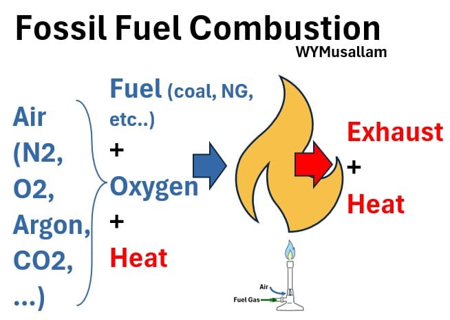
As I noted, Combustion is typically not complete and can produce several undesired byproducts. For example:
CO – Carbon Monoxide
SO2 – Sulfur Dioxide
Nitrogen Oxides – NOx , N2O
Volatile Organic Carbons VOCs, (e.g. Alkanes, Aromatics, Cyclic Hydrocarbons)
Particular Matter PM
Ammonia NH3
etc..
This means industry has to employ various technologies to reduce/eliminate these undesired by products (like low NOx burners, filters, cyclones, capture beds, etc.)
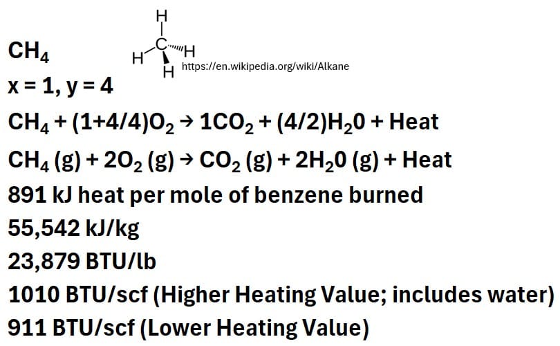
Example: Burning Methane
Natural Gas mostly comprises methane.
Its combustion formula is:
CH4 (g) + 2O2 (g) → CO2 (g) + 2H2O(g) + Heat ; Methane Combustion
Schematic: Methane Combustion
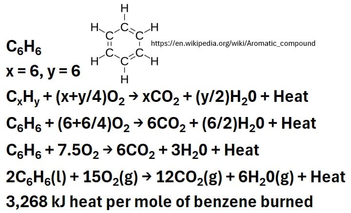
Example: Benzene Combustion
Benzene is a component of gasoline.
We can use the same exact combustion formula to derive the combustion equation for benzene.
C6H6 + 7.5O2 → 6CO2 + 3H2O + Heat; Benzene Combustion
Schematic: Benzene Combustion
Summary
Ok , so far, we know that:
- Dead animals and plants through millions of years of ‘hard work’ by the Earth are converted into liquid and gas hydrocarbons.
- Through amazing ingenuity and creativity, humans have figured out ways to extract these hydrocarbons from the Earth and
- utilize the energy from burning them to power our modern world.
- Complete combustion of hydrocarbons produces only carbon dioxide (CO2 ), water (H2O) , and heat.
- Incomplete combustion (and it will be incomplete in practice) produces undesirable molecules as listed above.
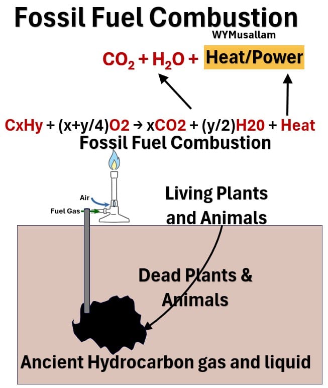
Fossil Fuel Combustion
Schematic – Fossil Fuel Combustion
CO2 is a greenhouse gas and a driver of global warming.
To understand how CO2 causes global warming, we have to first establish the foundational climate science governing energy and radiation.
The next several chapters build this framework. They’ll cover
- characteristics and composition of the Earth’s atmosphere,
- solar and terrestrial (Earth) radiation spectra,
- key Blackbody Radiation concepts like the Stefan-Boltzmann equation and Wien’s displacement law,
- Greenhouse gases,
- and Earth’s overall energy balance.
Once these physical mechanics are established, we will return to examine the carbon cycle in detail.
Earth’s Atmosphere
- Its Oxygen directly drives cellular respiration and energy production for living organisms.
- Nitrogen provides the reservoir that is fixed into ecosystems to build essential proteins and DNA.
- Water vapor and other greenhouse gases regulate the planet’s temperature.
- The ozone layer shields life from lethal solar UV radiation.
Let’s look at the detailed composition of air.
Air Composition
Gas/Symbol/Content
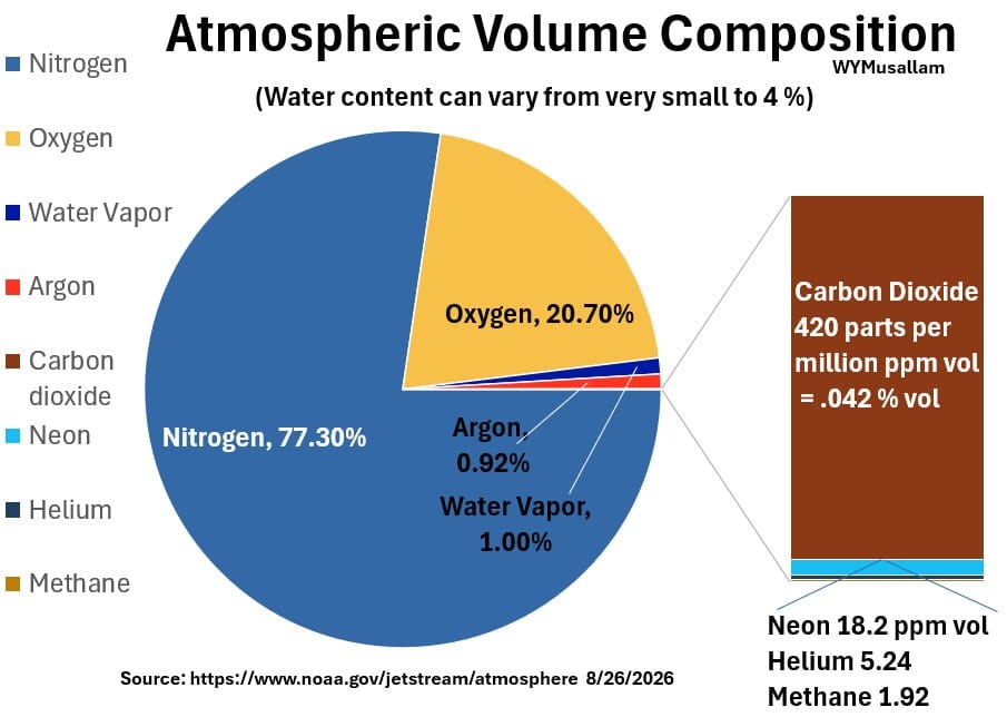
(Source: https://www.noaa.gov/jetstream/atmosphere)
Table: Atmospheric Volumetric Composition
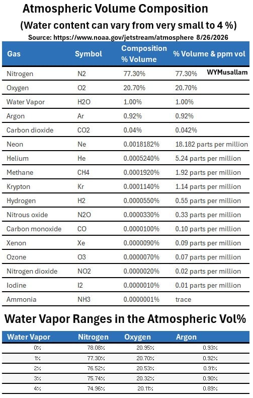
Chart: Atmospheric Volume Composition
Key Air Characteristics
- Water vapor in the air varies: It fluctuates from 0% to 4 vol % depending entirely on local temperature and geography.
- Almost all of water concentration is in the troposphere, the lowest 6 – 20 km layer of the Earth’s atmosphere (see picture below).
Picture: Atmospheric Layers
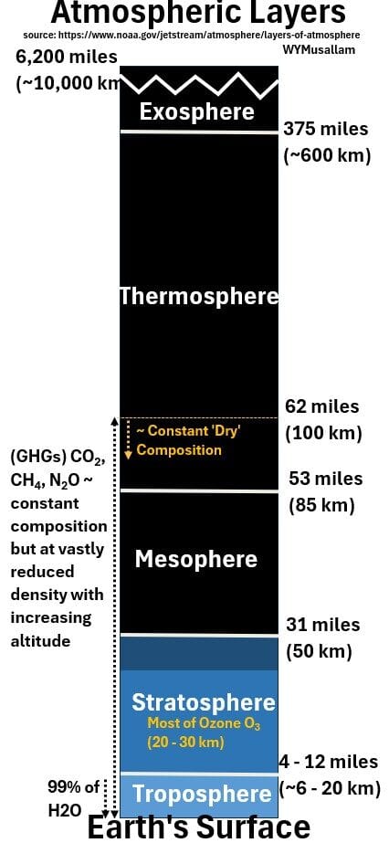
- Dry Air Composition (mass, molar) stays roughly constant up to 100 km into atmosphere (see picture above)
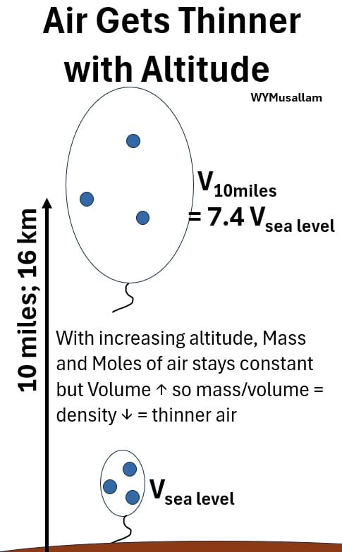
- But the density, the spread of the molecules, changes with altitude (see picture below using an expanding balloon analog).
- At higher altitudes, molecular interactions are not as frequent because they are more spread out (thinner atmosphere).
Picture: Air Gets Thinner With Altitude But Composition is Constant
- Certain air molecules (e.g. Carbon dioxide, Methane, Water vapor, Nitrous oxide, Ozone, and Chlorofluorocarbons) are called greenhouse gases (GHGs).
- The GHGs are the planet’s temperature regulators as they capture/trap/blanket heat on Earth.
- Non-GHG Gases dominate (N2, O2, and Argon make up 99% of total) but the GHG components of that remaining 1% (mostly water) are the climate regulators of our planet.
The atmosphere and its composition enables life on Earth (O2 for breathing, N2 for protein manufacture, warmth from greenhouse gases, and Solar UV protection from Ozone O2)
Before we learn more about greenhouse gases, we need to understand the types of radiation energy that the Earth receives and emits.
Electromagnetic Energy
- Electro Magnetic Radiation
- Electromagnetic waves – khanacademy
- Electromagnetic waves and the electromagnetic spectrum- khanacademy
Solar and Terrestrial Radiation
Of course, Earth gets its energy from the Sun.
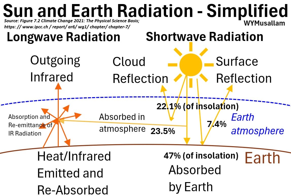
As shown in the simplified sketch below, radiation from the Sun enters the Earth’s atmosphere and is both reflected and absorbed.
- This incoming energy is called solar radiation (or shortwave radiation)
- About ≈30% of incoming solar radiation is reflected in the atmosphere (i.e. clouds) or off the surface of Earth while
- the rest of it (≈70%) is absorbed by the Earth (≈47%) and atmosphere (≈23%)
Source: IPCC Sixth Assessment Report – https://www.ipcc.ch/report/ar6/wg1/chapter/chapter-7/
The Earth itself emits radiation as well
- This emitted radiation form the Earth is called terrestrial radiation (or longwave / thermal Radiation)
Picture: Solar Radiation from the Sun and Infrared Radiation from the Earth.
The orange colored arrows in the picture above represent infrared radiation that is mostly sourced from heat and radiation emitted from the surface of the Earth.
- This radiation gets absorbed and re-emitted in the atmosphere, eventually either escaping to outer space or being re-absorbed on Earth.
- We’ll come back to this later after we discuss a few more foundational topics.
We need to review some wave properties next.
Wave Properties
Radiation is energy moving through space in the form of electromagnetic waves, which consist of oscillating electric and magnetic fields.
Electromagnetic waves can move through the vacuum of space, carrying radiant energy across the universe.
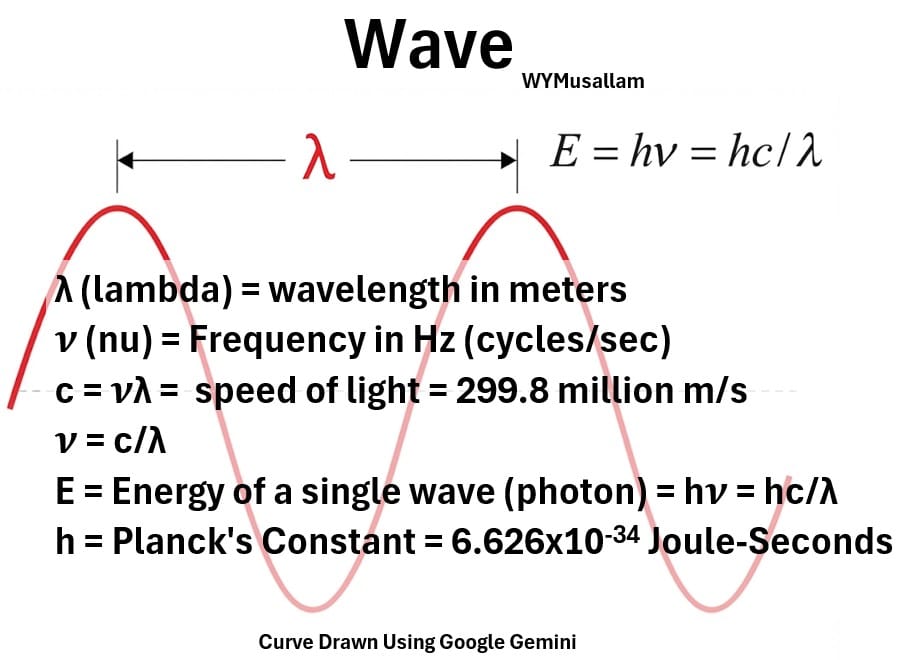
The properties of waves that we are interested in are shown in the schematic below.
Picture: Wave Characteristics
An electromagnetic wave has a
- wavelength (denoted with lambda λ; crest to crest or trough to trough distance) and
- frequency (denoted as nu ν; number of waves passing a point per unit time).
where
- λ (lambda) = wavelength in meters
- 𝝂 (nu) = Frequency in Hz (cycles/sec)
The product of wavelength and frequency produces a constant , the speed of light.
- c = 𝝂λ = speed of light = 299.8 million m/s
- 𝝂 = c/λ
Understanding Energy, Frequency and Wavelength
Building upon the wave nature of light, we can also examine its particle-like properties through energy.
While wavelength and frequency describe how a wave travels through space, Planck’s equation relates that a wave’s frequency 𝝂 directly to its energy:
Where:
- E = Energy of a single discrete packet—or quantum—of electromagnetic radiation, commonly known as a photon.
- h = Planck’s Constant = 6.626×10⁻³⁴ Joule-Seconds
- 𝝂 = Frequency in Hz (cycles/sec).
In this relationship, E describes the exact amount of energy carried by an individual photon.
We also know from above that the speed of light is equal to the product of its wavelength and frequency (c = λ𝝂):
Substituting for 𝝂 in Planck’s Equation give us E = hc/λ ; Planck’s Equation (as a function of wavelength)
Planck’s Equation shows that:
- Shorter wavelengths (such as ultraviolet light or X-rays) have higher frequencies and carry more energy per photon.
- Longer wavelengths (such as infrared light or radio waves) have lower frequencies and carry less energy per photon.
The Electromagnetic Spectrum
The electromagnetic spectrum encompasses the entire range of all types of electromagnetic radiation, organized continuously by wavelength, frequency, and energy.
- It ranges from low-energy radio waves and microwaves, through infrared, visible light, and ultraviolet, up to high-energy X-rays and gamma rays.
- Every type of radiation travels at the same speed of light , c,
- but each type of radiation differs fundamentally in its wavelength, frequency, and the amount of energy carried by each photon.
- In the picture below notice how as the wavelength λ decreases ( λ1 to λ2 to λ3), the frequency (𝝂 = Frequency in Hz (cycles/sec)) increases as well as the energy (indicated by the temperature).
Picture: Electromagnetic Spectrum
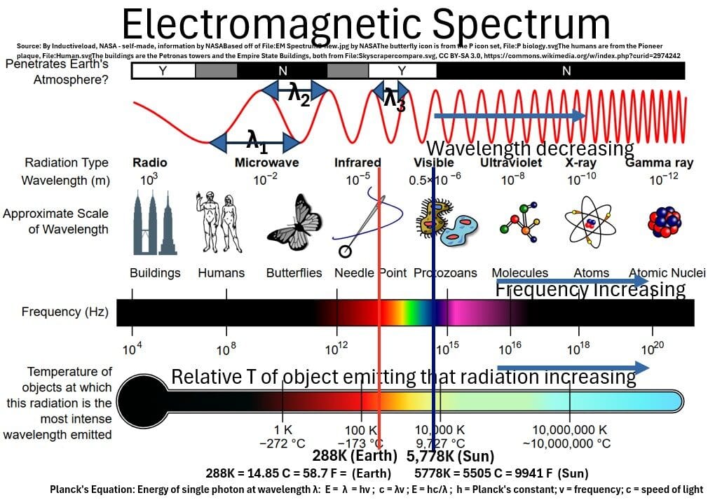
Consider the bottom temperature scale in the drawing above.
- This scale highlights a fundamental physical truth: all bodies with a temperature above absolute zero Kelvin continuously emit radiation.
- The higher the energy (frequency) , the higher the relative temperature of an object which is emitting that radiation.
- All objects will emit a defined continuous range of radiation which will vary in intensity.
- The Sun’s most intense radiation is in the visible spectrum while the Earth’s is in the infrared range.
- We will have a lot more to say on this in the section titled: Radiation from Bodies
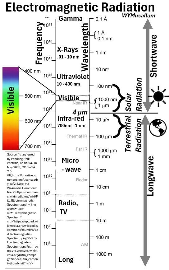
See the graph below to locate the solar radiation range and the Earth radiation range on a vertical electromagnetic spectrum.
- The solar radiation range goes from about .1 microns to about 3 microns
- The Earth radiation range extends from about 3 microns to 100 microns
- In climate science , we typically define 4 microns (4 micrometers or 4 μm or 4 x 10⁻⁶ meters) as the dividing point between shortwave radiation and longwave radiation.
- Often we describe the Sun’s and Earth’s radiation ranges as shortwave and longwave respectively.
Schematic: Solar Radiation and Terrestrial Radiation Ranges on the Electromagnetic Spectrum
Energy From The Sun
Inverse Square Law
In order for us to understand climate on Earth, we have to understand how much energy its receiving from the Sun.
Light energy must dilute in proportion to the expanding spherical area it travels.
The astronomer Johannes Kepler first articulated this in 1604.
Picture: Sunlight Irradiance and the Inverse Square Law
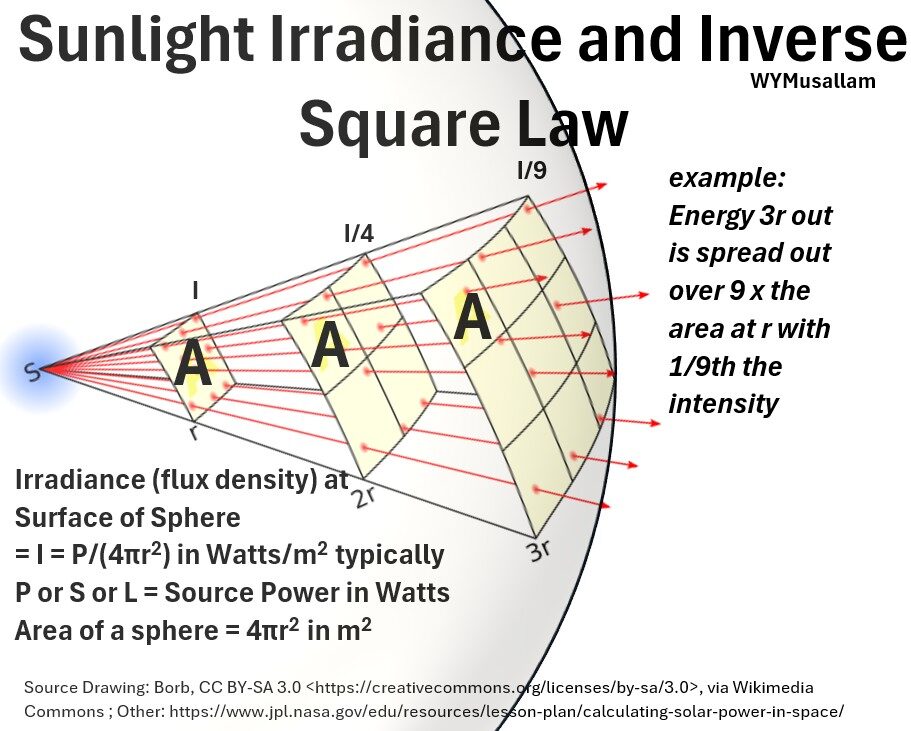
The total solar power (S for Solar power; or P for Power; or L for Luminosity) is the total radiant power (SI units = Watt = J/s) coming out of the Sun in all directions.
We can compute the amount of solar electromagnetic power (or radiant flux) received by a surface per unit area (the irradiance) as follows:
- I = Irradiance or flux density is the solar power received by a surface per unit area.
- Using the inverse square law, you take the Sun’s total output power (P), and spread it out over the surface area of an expanding imaginary sphere of radius r (4π r²) centered on the Sun.
- When that energy hits Earth, you are calculating how much power is arriving per unit area.
- Units of measure: Power per unit area (Watts / m² = W / m² ).
i.e. solar irradiance on a particular body in space is inversely proportional to the surface area of a sphere whose center is the Sun and whose radius is equal to the distance from that body to the Sun.
I = S / (4πr2)
where
- S = total solar power (S for Solar power; or P for Power; or L for Luminosity) = the total radiant power (SI units = Watt = J/s) coming out of the Sun in all directions.
- r = distance from Sun to object.
- For Earth r = 149.6 million kilometers (about 93 million miles) = 1 Astronomical Unit = 1 au
Today we use a tool called an Electrical Substitution Radiometer to measure solar irradiance at the top of the Earth’s atmosphere (about 400 to 800 km or 250 to 500 miles above surface of Earth).
For Earth, Isun-earth = 1361 Watts/m2
Isun-earth = 1361 Watts/m2; Solar Constant = Solar Irradiance (flux density) at the Top of the Earth’s Atmosphere
It is the average amount of solar electromagnetic radiation received per unit area at the top of Earth’s atmosphere, measured on a surface perpendicular to the Sun’s rays at a distance of one astronomical unit (distance from Sun to Earth).
So what is the value of S, the total solar power?
- The distance of the Earth from the Sun (astronomical unit) is 149.6 million kilometers (about 93 million miles).
- So we can calculate the total power of the Sun.
- S = Isun-earth4πr2
- S = (1361 W/m2)(4π)(1.496×1011 meters)2
S = 3.8275..x 1026 Watts = 383 trillion trillion Watts = 383 Septillion Watts
For our discussions I is the important number, but just be aware that S is just mind bogglingly large.
Average Power/m2 of Sun on Earth
Ok, we need to now average this solar constant (Isun-earth = 1361 Watts/m2 ) to the surface area of the Earth.
Check out my picture below as you read this section.
Picture: Average Solar Radiation is Solar Constant/4
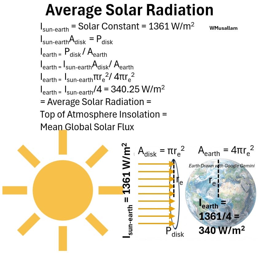
From the perspective of the Sun, the rays hitting the Earth are hitting a circular area with a radius equal to the Earth’s .
Imagine the light is a layer of paint spread out over this 2D Earth circle of area re.
- The total power in this circular area, Pdisk , on average, has to cover the whole surface area of the Earth.
- So, using the paint analogy, applying that layer of paint around the full sphere of Earth will thin it out or dilute it.
- So Iearth , the average solar radiation at Earth will be = Pdisk /area of the Earth
Let’s do the math and see what kind of expression we can get for Iearth
We know that,
Isun-earth = Solar Constant = 1361 W/m2
We can express the power of the Sun rays on that disk, in SI units of Watts, as Pdisk . This can be expressed as
1 . Isun-earthAdisk = Pdisk
where Adisk is the area of the circle with radius re (the radius of the Earth) that the light rays are hitting:
2. Adisk = πr2e
The Sun’s power in Pdisk must be applied across the whole surface area of the Earth.
3. Iearth = Pdisk / Aearth
Where
- Iearth = Average Solar Radiation = Top of Atmosphere Insolation = Mean Global Solar Flux
- Aearth = Surface area of the Earth as a sphere: 4πr2e
Substitute equations 1 and 2 and the expression for Aearth into equation 3 to get.
4. Iearth = Isun-earthAdisk / Aearth = Isun-earth πr2e / 4πr2e
This simplifies to
5. Iearth = Isun-earth / 4 = 1361/4 = 340 W/m2
= Average Solar Radiation = Top of Atmosphere Insolation = Mean Global Solar Flux
This will be useful when we compare the Earth’s spectral radiation to the Sun’s in a later section (We’ll need it to do Earth energy balances also).
The Sun’s Radiation Spectrum
The graph below is the theoretical (blackbody) spectral curve for the Sun which is generated using Planck’s Law.
Planck’s Law: Wavelength Form; Spectral Exitance/Emittance
Mλ(λ, T) = π · Lλ = (2πhc2) / (λ5 * (e(hc / λkBT)– 1))
Where
- Lλ = Spectral radiance as a function of wavelength
- Lν = Spectral radiance as a function of frequency
- λ = Wavelength of the light (measured in meters)
- ν = Frequency of the light (measured in Hertz)
- T = Absolute temperature (measured in Kelvin)
- e = The natural logarithm base (≈ 2.718)
- h (Planck’s constant) = 6.626 × 10⁻³⁴ J · s
- c (Speed of light) = 3.00 × 10⁸ m/s
- kB (Boltzmann’s constant) = 1.381 × 10⁻²³ J/K
Graph: Solar Radiation Spectral Curve
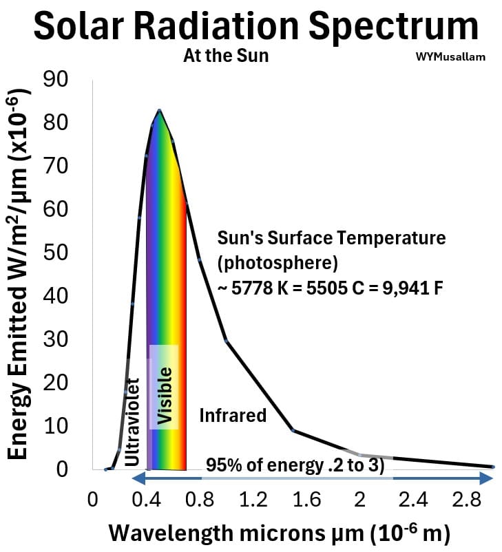
- While the equation is based on an ideal, theoretical emitter (a blackbody), it matches the Sun’s actual emission spectrum remarkably well.
- Of course we have modern instruments that can accurately measure solar radiation but Planck’s law gives an excellent approximation.
If you want to gain a solid understanding of blackbody concepts you should watch the videos referenced earlier and read Appendix 3 and Appendix 5.
Curves like these are called spectral curves or Planck curves or blackbody radiation curves.
Hot to Read Spectral Graphs
The x axis (abscissa = horizontal axis) indicates increasing wavelength from left to right
- Increasing wavelength means decreasing frequency (remember that c = hν).
- So we could have plotted the x axis as frequency, but in this article we will use wavelength.
The y axis (ordinate = vertical axis) of a spectral curve typically represents either spectral radiance or spectral radiant exitance (emittance).
Spectral Radiance measures how much power is emitted from a specific surface area, into a specific direction (solid angle), at a specific wavelength.
- See Appendix 5 and Appendix 6 for more details
- Spectral Radiance unit of Measure: W/{(sr)(m2)(m)} = Watts per square meter per steradian per meter of wavelength
- These are SI units. Typically you will see this in terms of microns or nanometers of wavelength: W/{(sr)(m2)(μm)} or W/{(sr)(m2)(nm)}
- A steradian is just a measure of a 3D cone of view (think of a sphere with 3D cone shape in it with top of cone on surface of sphere). See Appendix 5 for more information.
- 1 steradian equals a cone with an angular spread of about 65.5 degrees (a radian carves out about 57.3 degrees).
- Example: Imagine a 1 meter square hot plate. Spectral radiance measures the light of a specific color coming from one tiny dot on the hot plate straight into your eye from one exact angle.
- Spectral Radiance is sometimes described as the Intensity.
Spectral Radiant Exitance (Emittance) measures the total power escaping an entire surface across all directions in a hemisphere, per unit area, at a specific wavelength.
- See Appendix 5 and Appendix 6 for more details
- Spectral Radiant Exitance (Emittance) Unit of Measure: W/{(m2)(m)} = Watts per square meter per meter of wavelength.
- These are SI units. Typically the unit wavelength will be in micro meters or nano meters: W/{(m2)(μm)} or W/{(m2)(nm)}
- Example: Imagine a 1 meter square hot plate. Spectral radiant exitance measures all the light of a specific color spraying upward into the air from a one-meter square hot plate.
Ok, now that we understand these definitions, let’s get back to the spectral curve for the Sun in which we are plotting spectral radiant emittance W/{(m2)(μm)} versus wavelength λ in microns μm
Characteristics of the Sun’s radiation
- This curve is based on a body temperature of 5778 K = 5505 C = 9941 F which is the temperature of the surface of the Sun.
- The peak intensity is in the visible range (at a wavelength of about .5 microns)
- We typically see this as white light because it is a mix of all the visible colors.
- There is some ultraviolet as well as quite a bit of Infrared radiation as well
- As a percent of total energy we have roughly 7% UV, 44% Visible, 49% IR
- About 95% of the energy is between .2 and and 3 microns
Wien’s Law (Wien’s Displacement Law)
For the spectral curve of the Sun, for example, we can also compute the (ideal) wavelength at which the peak intensity occurs.
This is defined by Wien’s Law (Wien’s Displacement Law).
Wien’s law describes a simple rule about thermal radiation: the hotter an object gets, the shorter the wavelength where it shines the brightest.
- As temperature goes up, the peak of the radiation curve shifts to the left (toward shorter wavelengths).
- Example: A cool room-temperature object peaks far out in the invisible infrared; heat it up until it’s red-hot, and its peak shifts closer to visible light; heat it even more (like the Sun), and it peaks right in the middle of the visible spectrum.
λmax = 2897 /T ; Wien’s Law or Wien’s Displacement Law
where
- T is in units of Kelvin (T in Kelvin = deg C + 273) and
λ wavelength is in units of microns (μm = 1×10⁻⁶ meters)
So for example if we have the emission spectrum of a far away star, we can find the wavelength that corresponds to the peak intensity and plug it into Wien’s law to compute the temperature
- Example 1: Wavelength at peak emittance for Sun is about .5 microns. So T of surface of Sun = 2897 / λmax = 2897/.5 = 5794 K
We can of course compute for λmax as well.
- Example 2: Temperature of the Earth is on average about 59 F = 15 C = 288 K , so wavelength at max emittance λmax = 2897/288 = 10 microns
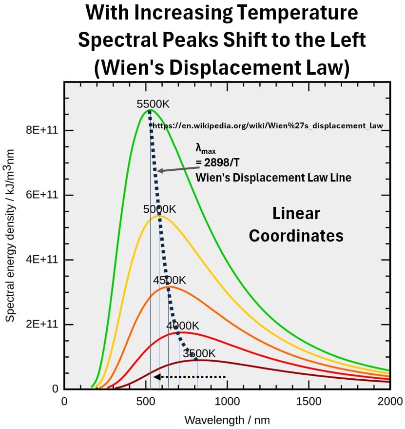
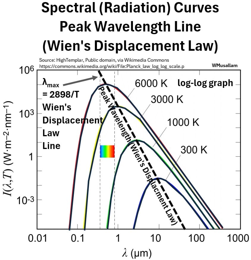
The two graphs below plot radiant emittance (radiant exitance) versus wavelength across several different temperatures, showing Wien’s law in action:
- The first Linear-Linear Graph shows the peaks sliding from right to left as temperature increases, following a curved displacement path.
- The second Log-Log Graph compresses the large number ranges so they all fit nicely on one page, turning the curved displacement line of the linear plot into a straight line.
Graph: Wien’s Displacement Law Shown on Spectral Curves with Linear Coordinates
Graph: Wien’s Displacement Law Shown on Spectral Curves with log Coordinates
Now consider the flame picture below (ie. in that visible light region shown in the graph above):
As the temperature of the flame gets hotter its color will shift from the red/orange region to the blue region.
Picture: Flame Colors

Ok, good, you understand Wien’s Displacement Law.
Let’s now look at the Earth’s radiation spectrum.
The Earth’s Radiation Spectrum
Using Planck’s Law to estimate the radiation spectrum of Earth, we get the graph below.
I’ll be redundant and show you the equation again (see Appendix 5 also and the reference videos provided earlier)
Planck’s Law: Wavelength Form; Spectral Exitance/Emittance
Mλ(λ, T) = π · Lλ = (2πhc2) / (λ5 * (e(hc / λkBT)– 1))
Where
- Lλ = Spectral radiance as a function of wavelength
- Lν = Spectral radiance as a function of frequency
- λ = Wavelength of the light (measured in meters)
- ν = Frequency of the light (measured in Hertz)
- T = Absolute temperature (measured in Kelvin)
- e = The natural logarithm base (≈ 2.718)
- h (Planck’s constant) = 6.626 × 10⁻³⁴ J · s
- c (Speed of light) = 3.00 × 10⁸ m/s
- kB (Boltzmann’s constant) = 1.381 × 10⁻²³ J/K
Graph: Earth Radiation Spectrum
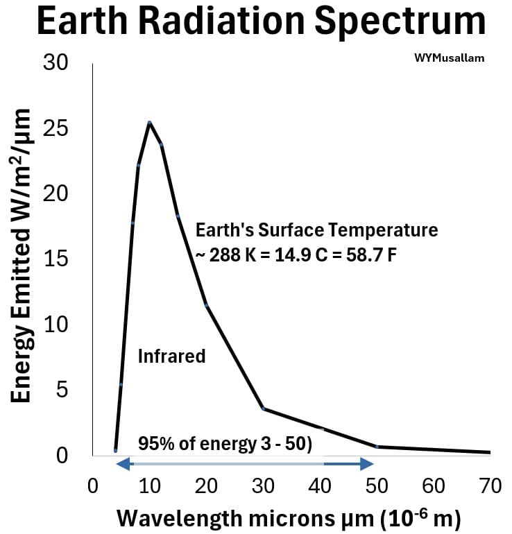
The shape is similar to the Sun’s but its energy and wavelengths are very different.
- The Radiant Emittance (Exitance) is much smaller than the Sun’s and
- peaks at about 10 microns (versus .5 microns for the Sun).
- The wavelengths are much larger than the Sun’s (lower energy) and are fully in the infrared electromagnetic region.
- When discussing the lower-energy, longer wavelengths of Earth’s emitted energy, we refer to this spectrum as thermal radiation (or outgoing longwave radiation).
- About 95% of the energy comes from wavelengths between 3 and 50 microns.
Earth and Sun Radiation Spectra Compared
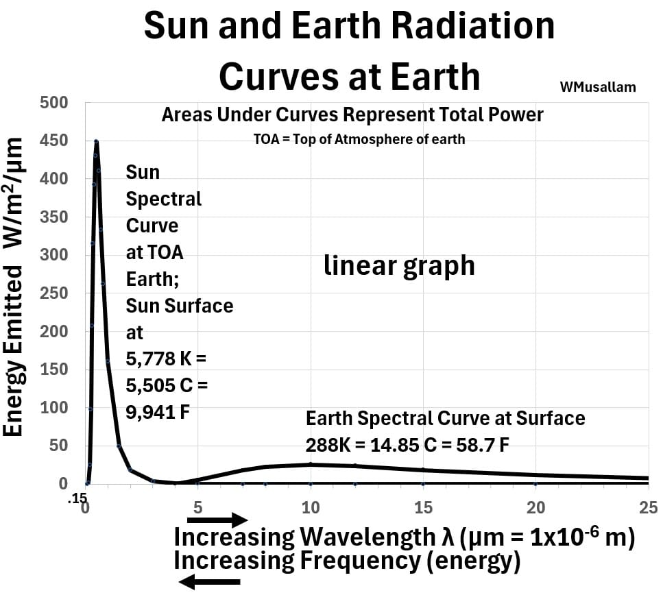
Let’s put the Sun’s and Earth’s spectral curves on the same graph.
You get the graph shown below.
- The location or measuring point for the Sun’s rays is the top of the Earth’s atmosphere (TOA; about 400 to 800 km or 250 to 500 miles above surface of Earth)
- while the Earth’s measuring point is at its surface.
Graph: Spectral Curves for Sun and Earth (linear graph)
What the Curves Tell You
- The Sun’s curve skews to the left (uv/visible/ir range) and peaks much higher than the Earths curve. This indicates its high surface temperature (5778 K)
- Earth’s curve is tiny in terms of energy emitted per wavelength and shifted far to the right into the thermal infrared because Earth is much cooler (288 K on average). This is a direct visual proof of Wien’s law.
- The two curves barely overlap. A common dividing line is about 4 microns.
- The Sun emits almost entirely in short wavelengths, while Earth emits entirely in long wavelengths.
- Due to this gap in wavelength ranges and the presence of the Earth’s atmosphere, the Earth is able to maintain livable temperatures (more on that later).
What the Area Under the Curves Tells You
When you plot spectral emittance against wavelength on the x-axis, finding the area under that curve is the same as taking the integral across all wavelengths.
Mathematically, that looks like this:
Total emittance = ∫0→∞E λdλ (see my article on integration)
- The areas under the curves represent the total radiant emittance/exitance in units of power/area (SI units: W/m2 )
- Recall that the Sun’s irradiance hitting our upper atmosphere to be about 1,361 W/m2
- Also recalled from a previous section how we computed the average solar radiation relative to the Earths surface as Iearth = Isun-earth / 4 = 1361/4 = 340 W/m2
So, the area under the solar curve represents this average solar radiation (irradiation) of 340 W/m2
The area under Earth’s curve represents the total thermal energy Earth radiates from its surface.
If we assume the Earth’s average surface temperature is 15C, then the Stefan-Boltzmann equation gives us a total emitted energy of about 390 W/m2
Eearth = εσT4 (Stefan-Boltzmann Equation) = (ε=1)(σ =5.670 × 10⁻⁸ W/m2/K4)(T = 15 + 273 K)4 = 390 W/m2
The curves in the linear graph above are visually hard to understand/compare with respect to area, so a clever way to plot the same data points is shown in the graph below
Graph: Spectral Curves for Sun and Earth (linear – log2 graph)
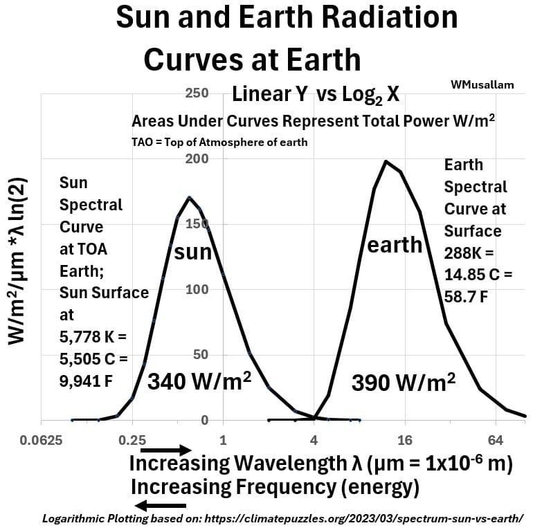
The graph above plots Radial Exitance (Emittance) * λ * ln(2) vs λ on a linear (Y axis) vs log base 2 scale (X axis).
Multiplying the axis by λ * ln(2) and plotting it against the log base 2 of the wavelength produces two bell shaped curves with much more “visibly comparable” areas underneath them.
I created this in excel using Planck’s and then adjusting the Y axis value and then plotting the x axis as log base 2.
Cool. The curves now look like symmetrical bell shapes with areas that exactly represent the total energy of each one.
The linear Sun curve has essentially been stretched out on the x axis and the Sun’s wavelength range has been compressed.
Keep these key comments in mind:
- The linear-linear plot is the one to use to see the real shape and distribution and to locate max λ (i.e. Wien’s Displacement Law)
- The linear-log2 curve does not correlate directly to either Planck’s Law or Wien’s Displacement law, but it does show an accurate visual depiction of the total energy of the Sun, Power/area, (at TOA of Earth) vs the Earth (at surface).
See Appendix 4 and Appendix 8 for more details on these graphs and what they mean.
I was able to generate the linear log graph using this reference:
Now, you might have been scratching your head looking at the linear-log graph above and noticing that the Earth area is larger than the Sun area.
Total Esun ≈ 340 W/m2 and total Eearth ≈ 390 W/m2, i.e. Earth total E is about 15% larger.
How can that be?
- Well, remember we have defined total Esun at the top of atmosphere of Earth.
- At the surface of the Sun its area would make the Earth area disappear on the same graph (i.e. it’s orders of magnitude bigger).
- You should actually expect them to be the same since the energy of any body in equilibrium should have matching incoming (Sun) and outgoing (Earth) energy
By the First Law of Thermodynamics, a body in steady thermal equilibrium cannot accumulate or lose net energy over time, or its temperature would change.
Therefore, the rate of incoming energy absorbed should precisely balance the rate of outgoing energy emitted.
But the graph above does not show equal areas. What is going on?
Two things explain this: (1) the measuring locations for the Sun and Earth spectra and (2) the atmosphere
Read on.
Calculating the Average Earth Surface Temperature (Ignoring the Atmosphere)
Assume Average Earth Temperature is Constant
The First Law of Thermodynamics states that energy cannot be created or destroyed.
For any defined system, the change in stored energy must equal the net difference between what enters and what leaves.
Applying this to Earth,
- Energy In is shortwave radiation absorbed from the Sun.
- Energy Out: Longwave thermal radiation emitted from the Earth back into space.
- Change in Stored Energy = Energy In – Energy Out
- If the temperature of the Earth is constant, the change in stored energy is zero.
- This means that Energy in = Radiation In = Energy Out = Radiation Out
Assume for now that the Earth is , on average, at a constant temperature so it automatically radiates heat away at the exact rate it absorbs it.
Now consider the Sun rays entering the Earths atmosphere (Top Of Atmosphere, TOA, about 400 to 800 km or 250 to 500 miles above surface of Earth)
Energy from The Sun at Earth’s Top of Atmosphere
We want to know the solar energy the Earth is getting from the Sun.
We computed this using the inverse square law in the “Energy from the Sun” section:
- Iearth = Isun-earth / 4 = 1361/4 = 340 W/m2
- = Average Solar Radiation
- = TOA (Top of Atmosphere) Insolation
- = Mean Global Solar Flux
- This is the total power /m2 at the top of the atmosphere (TOA) of the Earth.
As this average power of 340 W/m2 enters the Earths atmosphere and moves towards the surface of the Earth some of it is reflected right back out to space.
Albedo = Whiteness = Surface Reflectivity
As sunlight enters the atmosphere some of it is reflected by clouds and some gets reflected off the Earth itself.
In total about 30% of incoming sunlight is reflected back out into space.
We measure this as reflectivity or Alebedo (pronounced Al Bee Dough), the proportion of light reflected from a surface:
- Comes from the Latin, albus, meaning white
- Coined by the Swiss scientist Johann Heinrich Lambert in 1760
Picture: Albedo is % Surface Reflectivity
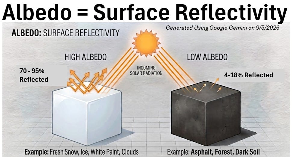
Typical Albedos are listed below.
Surface Material / Albedo Range/ Albedo Average
Data Sources: National Renewable Energy Laboratory (NREL) SURFRAD database, PVsyst meteorological solar databases, and standard geophysical literature compiled via Pennsylvania State University (EARTH 103) and MeteoSwiss.
- Fresh Snow/ 0.80 – 0.95/ 0.85 (85%)
- Old / Melting Snow/ 0.40 – 0.80/ 0.55 (55%)
- Cumulonimbus Clouds/ 0.70 – 0.90/ 0.9 (90%)
- Stratocumulus Clouds/ 0.30 – 0.60/ 0.6 (60%)
- Desert Sand / Quartz/ 0.35 – 0.45/ 0.4 (40%)
- Light Concrete/ 0.30 – 0.50/ 0.35 (35%)
- Grasslands / Green Grass/ 0.18 – 0.25/ 0.2 (20%)
- Deciduous Forest/ 0.15 – 0.18/ 0.17 (17%)
- Coniferous Forest/ 0.08 – 0.15/ 0.12 (12%)
- Ocean Water/ 0.05 – 0.10/ 0.07 (7%)
- Fresh Asphalt/ 0.04 – 0.12/ 0.08 (8%)
- Whole Earth (Average) – 0.30 (30%)
So ,no surprise, snow and clouds have high albedo and reflect a large percent of sunlight that hits them.
Notice that forests and oceans have very low albedos (they absorb much of the sunlight).
On average the Earth’s albedo is about 29.5%.
The Earth’s albedo or reflectivity influences the reflection we see in the drawing below (at Earth and in atmosphere above Earth from clouds mainly).
Let’s take that simplified picture we introduced some sections ago and show it a little differently.
Picture: Radiation Paths on Earth
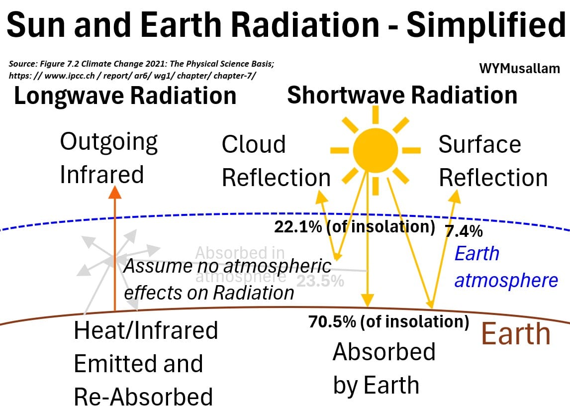
For now, let’s assume there is no atmospheric absorption or re-emittance (which we will explore soon).
We just assume we have solar radiation coming in with about 29.5% (lets round this off to 30%) being reflected (and about 70% being absorbed)
Average Surface Temperature of Earth as a Blackbody
Let’s now calculate the average temperature of Earth at its surface, assuming no atmospheric effects.
We’ll use our good friend , the Stefan-Boltzmann Equation:
- E = εσT4 ; Stefan-Boltzmann Equation
- E (Total Emissive Power): The total energy emitted per square meter of the surface per second, measured in Watts per square meter W/m2.
- ε (Emissivity): an efficiency comparing a real body to an ideal blackbody radiator ; It’s a decimal between 0 and 1 (or 0% to 100%).
- σ (Stefan-Boltzmann Constant): A fundamental universal physical constant: 5.67×10⁻⁸ W/(m2 K4)
- T4 (Temperature to the Fourth Power): The absolute temperature of the object measured in Kelvin (K), raised to the 4th power.
We can now express an energy balance: Solar Radiation Energy into Earth = Radiation Energy Emitted From Earth (which should be true on average if the temperature is constant)
ETOA (1-Albedo) = εσTearth4 ; Earth Energy Balance (Simplified; No Atmospheric Absorption or Re-emittance effects)
The average emissivity of Earth’s surface across land, oceans, and ice is very high, typically ranging between 92% and 98%, meaning the ground and water act as near-perfect blackbody radiators.
So let’s plug in all our known values and assume that ε ≈ 1.
340 (1-30%) = 238 W/m2 = (1)(5.67 x 10⁻⁸)(T4)
and solving for T we get
T blackbody earth surface = 254.53 K = (254.53 – 273.15)C =-18.62C = -1.52 F ; Assuming No Atmospheric Absorption
Well, that is not correct! We know the average Earth temperature is higher than that.
We’ve measured temperatures in Antarctica as low as -128.6F = -89.2C, but,
if the average Earth temperature was -18.62C, all living things would not exist (perhaps excluding tiny microbes living deep in the sea).
The assumption we made about “no atmospheric absorption effects” must be the reason.
- Without Earth’s atmosphere, humans would be f***ed.
- Without it, the Earth is a big solid ball of ice.
We need to discuss atmospheric absorption effects of course, which means we need to talk about greenhouse gases.
Greenhouse Gases (GHGs) References
- Greenhouse effect and greenhouse gases – khanacademy
- The greenhouse effect – khanacademy – Mahesh Shenoy
- https://www.climate.gov/ghg/what-are-greenhouse-gases-and-why-do-they-matter
- https://www.epa.gov/ghgemissions/overview-greenhouse-gases
GHGs
Greenhouse gases (GHGs) in our atmosphere, such as carbon dioxide, methane, water vapor, and nitrous oxide, possess specific molecular symmetries and uneven charge distributions that allow them to resonate with infrared frequencies.
That is to say, GHGs will selectively absorb thermal radiation wavelengths (between roughly .4 and 100 microns).
Recall from the graph below from the “Earth and Sun Spectra Compared” section, that this wavelength range
- coincides with Earth’s emitted infrared radiation and
- excludes the Sun’s shorter spectral range.
Picture: Sun and Earth Spectral Curves at Earth (Linear-Linear)
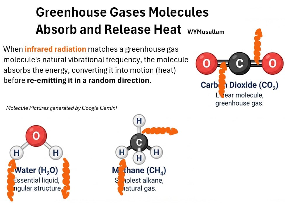
When these GHG molecules absorb this thermal radiation, they vibrate and instantly re-emit that energy in all directions, effectively trapping heat within the atmosphere
If you want to learn more about the mechanism you should research the topic of IR spectroscopy.
- https://teachersinstitute.yale.edu/curriculum/units/1999/5/99.05.07/4 – See the section on molecular vibrations
- listen/watch at 8:36 in the Mahesh Shenoy video above
Recall from the “Earth’s Atmosphere” section that the atmospheric composition (up to roughly 100 km above the Earth and about 20 km with respect to water), is mostly made up of nitrogen and oxygen.
- Major atmospheric components like nitrogen (N2) and oxygen (O2) are symmetric diatomic molecules
- that let thermal radiation pass freely into space (i.e. they don’t absorb, vibrate, and re-emit infrared radiation).
But, certain greenhouse gas (GHG) molecules found in the air in smaller concentrations (like water, carbon dioxide, methane, and nitrous oxide), act like a thermal blanket, capturing Earth’s outgoing energy and warming the lower atmosphere.
In the sketch below, I illustrate how an incoming Infrared electromagnetic wave can be absorbed by a GHG and then get re-emitted in any direction, with some IR getting routed back downward.
It’s this capture effect (the downward re-emittance) that we describe as the warming Greenhouse Effect.
Picture: GHGs Absorb Infrared Radiation and Then Re-emit it in any direction
You can refer to Appendix 2 for more information on the impact and sources of these GHGs.
Earth’s Effective or Global Radiative Transmittance
Despite making up a minuscule fraction of an atmosphere dominated by nitrogen and oxygen, greenhouse gases (GHGs) massively affect the Earth’s energy balance.
They allow 60% of the Earth’s thermal radiation escape to outer to space; a metric known as global or effective atmospheric transmissivity; while intercepting and recycling the remaining heat.
So, in the picture below, which we’ve seen before:
- some portion of the Sun’s radiation is absorbed by the Earth (the yellow arrow hitting the Earth) and
- then Earth emits infrared energy which (mostly) gets absorbed and then re-emitted GHG molecule including water.
- The energy of a hypothetical single emitted ray from the Earth is mostly absorbed and re-emitted and again re-absorbed and re-emitted throughout the atmosphere (as the rays hit other GHG molecules).
- This cascading effect continues until a smaller fraction of that energy, roughly 60%, (of that total initial ray of energy that left the Earth) escapes to outer space.
- And into this we add the complexity of some insolation that is also absorbed in the atmosphere.
- We say the effective or global transmittivity of the Earth τ is 60%.
Let’s introduce our simplified energy balance picture again , but we now show both solar and Earth radiation being absorbed and re-emitted in all directions,
- where some longwave radiation escapes the atmosphere
- and some is re-absorbed by the Earth.
Picture: Radiation Paths on Earth
We need to add a little more detail to this picture to see what climate scientists have determined to be a reasonable Earth energy balance.
Earth’s Average Energy Balance
Source: IPCC Sixth Assessment Report – https://www.ipcc.ch/report/ar6/wg1/chapter/chapter-7/
The picture below gives us a more detailed view of the Earth’s average energy balance:
Picture: Earth Average Energy Balance
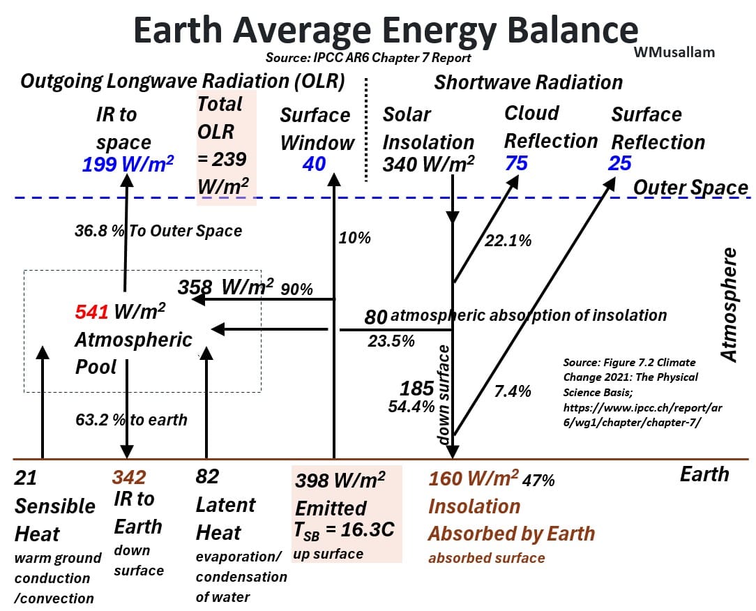
The picture above shows a balance of Sun energy (longwave radiation) entering the Earth’s atmosphere and Earth Energy (in the form of longwave radiation) exiting the Earth and the atmosphere.
- All values shown are energy rates in Watts/meter squared = W/m2
- The picture shows the Earth’s surface and the atmosphere / outer space boundary.
- Energy is entering our atmosphere from the Sun and leaving as infrared radiation into outer space (Outgoing Longwave Radiation or OLR).
- Solar energy is reflected and absorbed in the atmosphere and absorbed by Earth.
- Recall from the “Energy from the Sun” section that 340 W/m2 is the average solar radiation = top of atmosphere insolation = mean global solar flux.
- So Sun energy (solar insolation or shortwave radiation) comes in at 340 W/m2.
- About 29.5% of the energy from the Sun is reflected (called Albedo), 23.5% is absorbed directly by the atmosphere, and the remaining 47% is absorbed by the Earth.
- The Earth radiates 398 W/m2 of infrared radiation , about 10% of which (40 W/m2 ) escapes directly to outer space with the vast majority getting absorbed in the atmosphere (358 W/m2).
- Also entering the atmospheric pool of energy is 80 W/m2 of solar radiation.
- Latent heat and sensible heat enter the atmospheric pool from the Earth.
- Latent heat is constant temperature heat transfer of evaporating and condensing water.
- Sensible heat transfer is the (temperature changing) direct thermal conduction and convection from the warm ground into the lowest air layer.
- About 36.8% (199 W/m2) of the atmospheric radiation pool escapes to outer space while about 63.2 % of it (342 W/m2) gets re-absorbed into the Earth
So what does this all tell us? Well, the balance shows that
The Earth emits 398 W/m2 but only rejects 239 W/m2.
About 60% (239/398) of the Earth surface emitted radiation is ejected into space with 40% (~159 W/m2) being captured by GHG molecules in the atmosphere.
As we noted before, this value of 60% is sometimes called the global or effective atmospheric transmissivity.
We can designate this as τ and incorporate into the Earth energy balance:
Recall we the Stefan-Boltzmann equation to compute the Earth’s blackbody (ideal) temperature: ETOA (1-Albedo) = εσTearth4
Lets modify it with the global transmissivity factor τ:
Eincoming from the sun = Eoutgoing from the earth
ETOA(1-Albedo) = τεσT4earth ; Earth Energy Balance
Where
- ETOA = 340 W/m2 = Average Solar Radiation Energy at top of Earth in W/m2
- Albedo = 29.5 % reflectivity of Earth
- τ = Average Global Transmittance of Earth = about 60%; Fraction of Earth emitted radiation that escapes to space
- ε = Emissivity = an efficiency comparing a real body to an ideal blackbody radiator ; Earth’s is roughly equal to 1.
- σ = Stefan-Boltzmann Constant = 5.67 x 10⁻⁸ W/(m2 K4)
- T4 earth = Earth surface temperature to the Fourth Power in Kelvin (K); Deg C + 273.15 = K
Using the equation above Tearth = 61.3 F (16.3 C) ; Idealized average surface temperature for Earth
- Of course, we could have also computed this by solving the Stefan-Boltzmann equation for T using E = 398 W/m2
That temperature of 61.3 F (16.3C) makes more sense. We have liquid water and we have life on Earth.
Correcting Our Calculation for Latent and Sensible Heat Earth Cooling
We need to make a correction to our calculation in order to account for cooling effects from latent and sensible heat surface effects.
The calculation above assumes that thermal radiation (infrared light) is the only way energy leaves Earth’s surface.
- Under pure radiation, modern flux values yield a theoretical surface temperature of 16.3 C (the value we calculated above).
- This is for a 398 W/m2 emittance from Earth where 60% of it escapes through the atmosphere.
In reality, Earth also cools by “sweating” (evaporation) and rising warm air currents, which strip over 100 W/m2 directly off the ground (82 W/m2 latent heat and 21 W/m2 sensible heat) .
This non-radiative cooling pulls Earth’s actual modern average surface temperature down to 15.0C,
which is up from the pre-industrial baseline of 13.7 C – 14.0 C before 1.2 to 1.3C of post-industrial warming.
We could have also made this adjustment by changing the transmittivity tau from 60 to about 62%.
This seems like a tiny temperature spike relative to the temperatures the average human experiences in a year.
It’s actually very significant, but we’ll address this later on in the article after we establish some more foundational knowledge.
Earth Average Temperature Summary:
In a world where the atmosphere is not absorbing any radiant heat, the Earth’s average temperature would be about -18.6 C (-1.5 F).
In reality, accounting for the warming effects of the atmosphere and assumed reflectivity, Earth’s average temperature is about 15 C (59 F).
The atmosphere, due to its greenhouse gases warms the Earth by about (15 – – 18.6 ≈ 33.6 C = 92.5 F).
This is called the Greenhouse Effect
According to Nasa ,
- Water vapor H2O accounts for about 50 percent; and
- Clouds (H2O) account for 25 percent.
- i.e. About 75% from water alone
- Carbon dioxide CO2 causes about 20 percent of Earth’s greenhouse effect;
- The rest is caused by small particles (aerosols) and other greenhouse gases like methane CH4.
So, Water is the biggest warming contributor but CO2 and CH4 are the ones we are concerned with (and to a lesser degree the other GHGs).
- While water vapor traps the most heat, it rains out in days and merely amplifies existing temperature changes.
- Carbon dioxide , CO2 , is the primary gas of concern because it stays in the atmosphere for centuries, acting as the “thermostat” that drives global warming and dictates how much water vapor the air can hold.
- Methane has a shorter atmospheric lifetime; approximately 12 years on average. But it still has a significant warming effect. (https://ghginstitute.org/2024/10/17/which-methane-gwp-value-do-i-use/)
More on greenhouse gases later.
Calculating a global average energy balance was necessary to show how the atmosphere as a whole traps heat and sets Earth’s baseline temperature.
However, temperatures obviously vary widely across the planet, and no single location actually lives at 15°C.
To understand where this energy accumulates and how it moves across the globe, our next step is to examine the latitudinal energy balance.
Earth’s Latitudinal Energy Balance (Wind and Waves)
We know that an average Earth temperature is really useful when doing overall (macro) energy balances and trying to understand global warming.
Yeah there are probably places like California that might have an average yearly temperature pretty close to the Earth’s average but in generally we all know that the planet’s temperatures are not equally distributed.
Earth’s latitudinal energy balance describes the fundamental heat imbalance created by Earth’s spherical shape:
- the tropics absorb a massive solar energy surplus, while
- the poles run a continuous thermal deficit.
To prevent the equator from endlessly overheating and the poles from freezing solid, planetary winds and ocean currents act as a global engine that constantly pumps excess heat toward higher latitudes.
This continuous redistribution of thermal energy is the primary driver behind all global weather systems, ocean circulation, and the overall habitability of the planet.
This section gives a “schematic heavy”, “text light” outline description of the unequal temperature distribution and its implications.
To see a more detailed version of the below please review
Appendix 9 : Climate Science Basic Physics
- Understand why hot air rises via the ideal gas and Archimedes’s Law (Buoyancy Law).
- Understand what mass flux and heat flux mean
Appendix 10 : Latitudinal Energy Balance
- A detailed description of the outline that follows.
Outline of Latitudinal Energy Balance
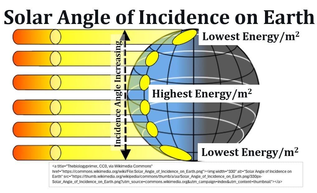
Unequal Heating: Earth’s curvature concentrates solar radiation at the tropics and spreads it thin near the poles.
Picture – Solar Angle of Incidence on Earth
Average Annual Temperatures Vary by Latitude.
Graph: Latitudinal Raw and Area Weighted Mean Annual Temperatures

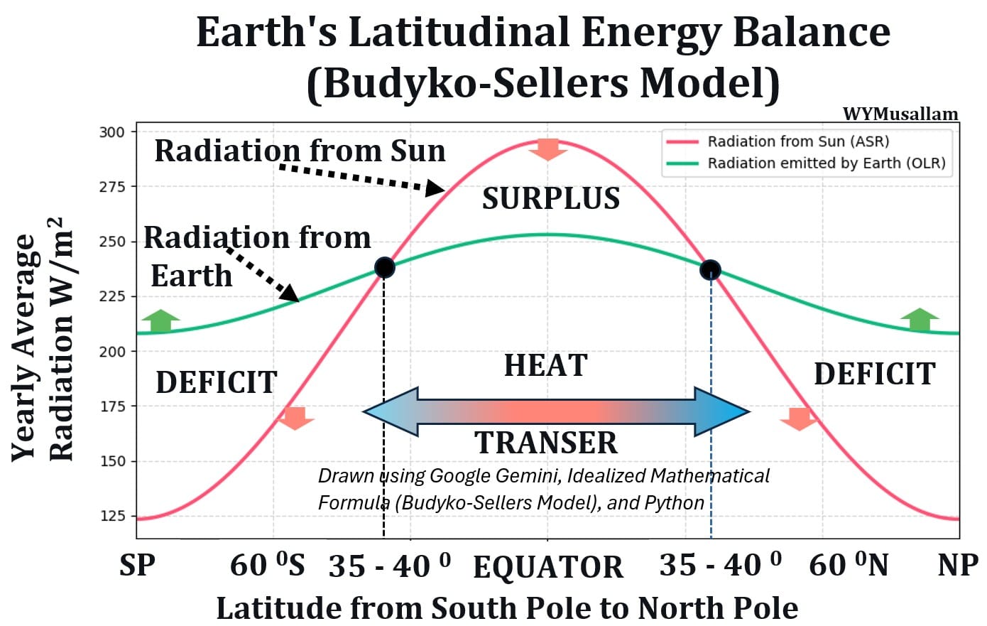
Energy Imbalance: Latitudes within 35° N/S hold a thermal heat surplus, while high latitudes run a deficit.
Heat Transfer away from the Equator to the Poles prevents infinite heating and cooling.
Graph: Earth’s Latitudinal Energy Balance
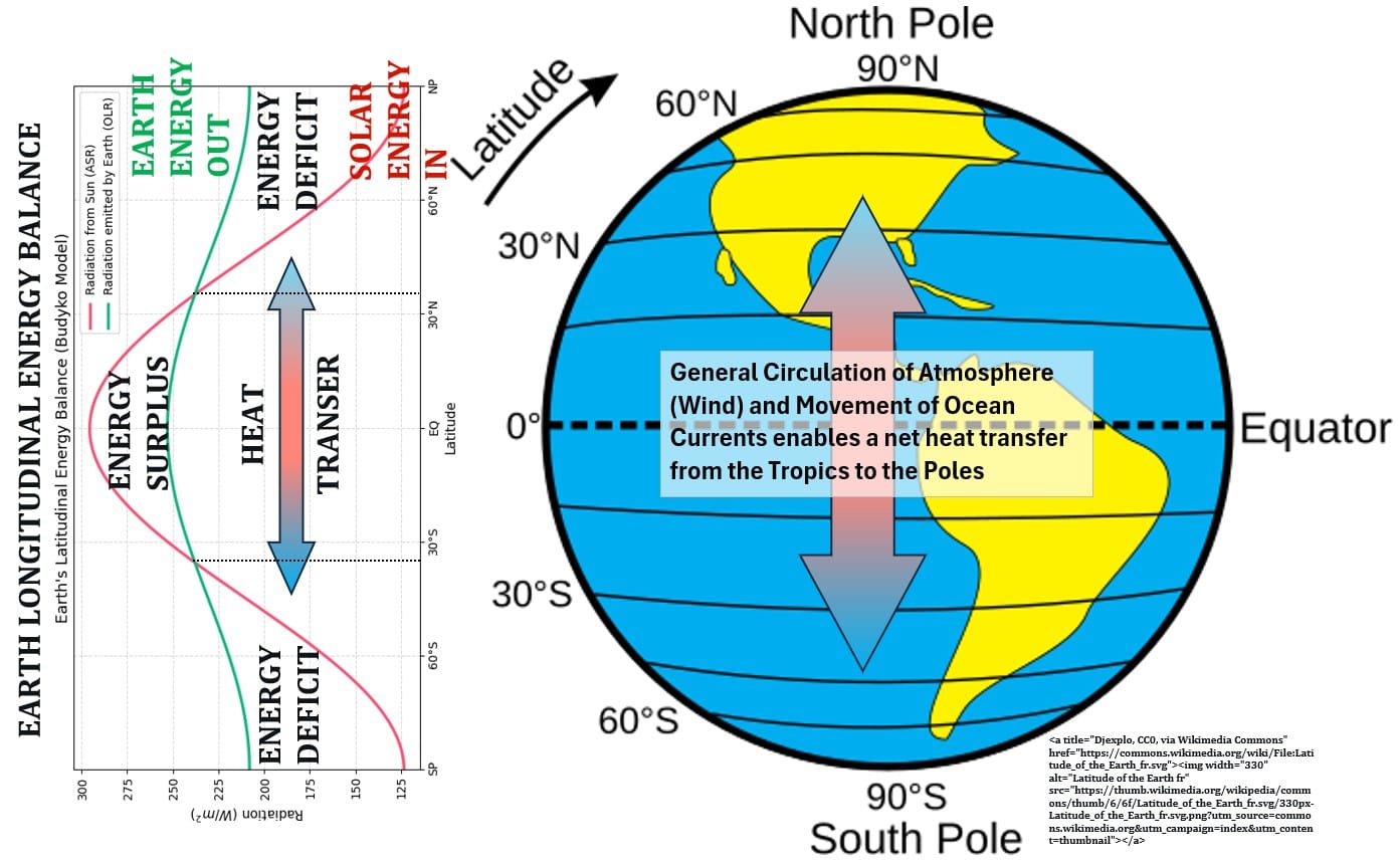
Heat Transport: Planetary winds and ocean currents continuously move surplus equatorial heat toward the cold poles.
Picture: Latitudinal Energy Balance Graph overlayed with Picture of Earth’s Latitudes
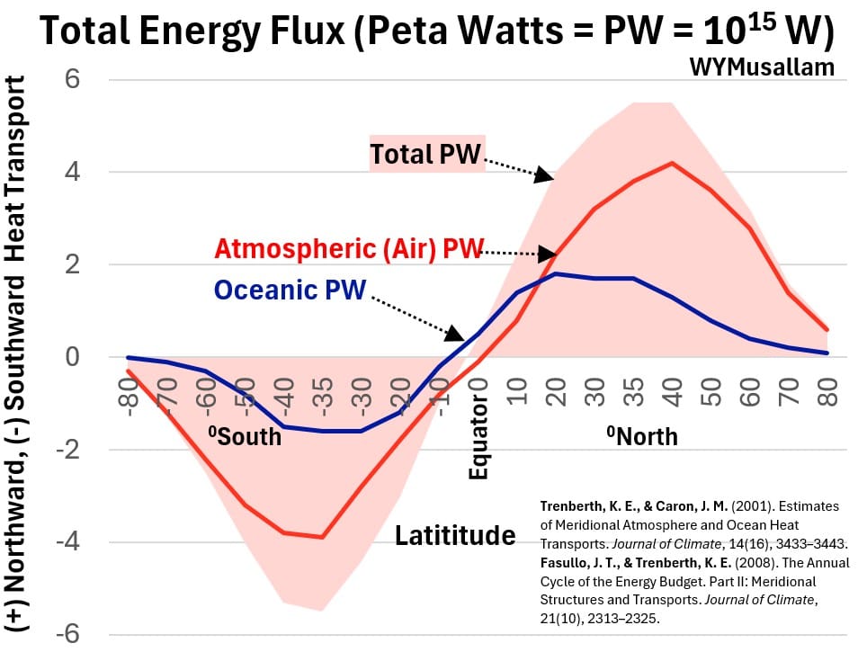
Workload Split: Oceans move most heat in low latitudes (10°–20°), while atmospheric winds dominate in mid-to-high latitudes.
Graph: Northward/Southward (towards Poles) Movement of Energy
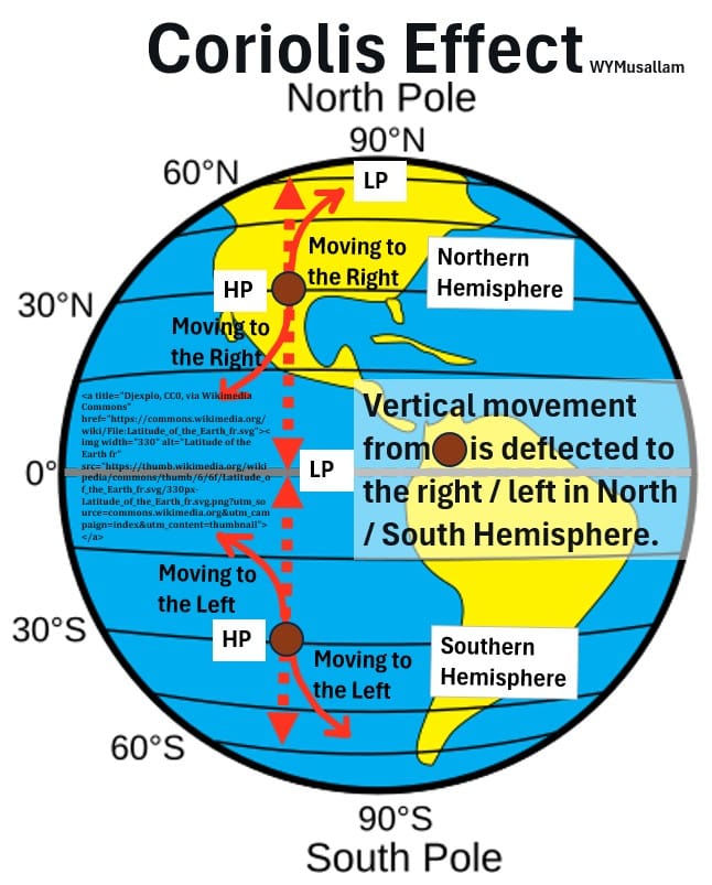
Wind and current (ignoring effects of land masses) would have a north and south movement if it wasn’t for the spinning of the Earth.
Coriolis Effect: Earth’s spin deflects moving air and water to the right in the Northern Hemisphere and left in the Southern.
Picture: Coriolis Effect
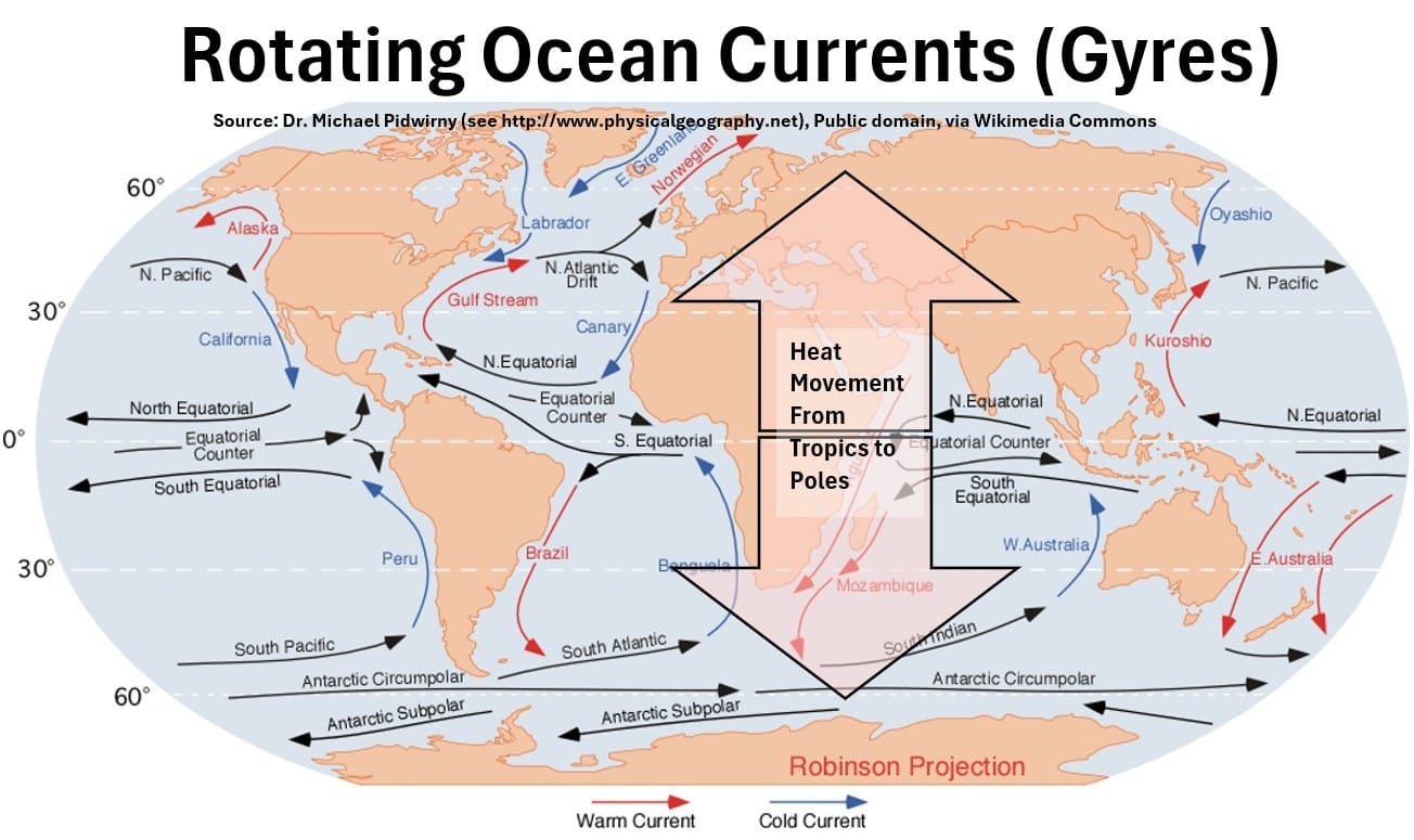
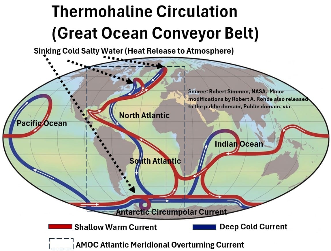
Ocean Circulation: Surface winds form rotating gyres, while temperature and salinity drive deep 3D currents (like AMOC).
Picture: Rotating Ocean Currents (Gyres)
Picture: Deep Sea Circulation – Thermohaline Circulation (Great Ocean Convery Belt)
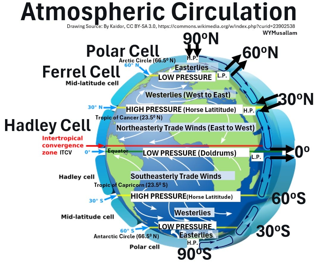
Atmospheric Cells: Three convection loops per hemisphere (Hadley, Ferrel, Polar) create global wind belts and calm zones (Doldrums, Horse Latitudes).
Picture: Atmospheric Circulation (Convection Cells, Winds, High and Low Pressure Areas)
That is a lot. Climate 101. It’s basic physics though i.e. “things tend to balance”.
Let’s now take a closer look and compare the greenhouse gases and explore their impact on global warming.
Contributions to Global Warming from Various Greenhouse Gases
Our average energy balance in a previous section shows that the net capture of radiation in our atmosphere is about 159 W/m².
The table below shows how water and other greenhouse gases contribute to this.
Table – Contributions to the Greenhouse Effect
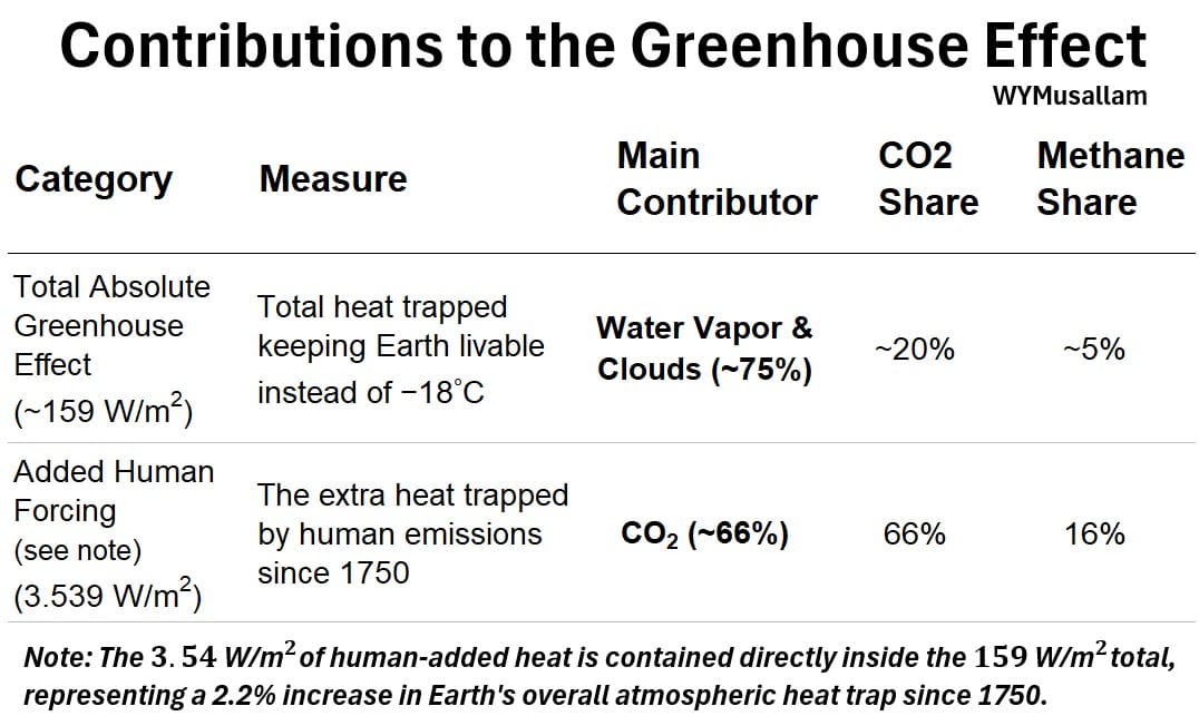
Climate scientists define radiative “human” forcing (see this NOAA article or this MIT article) as the heat capture caused by man made greenhouse gases.
- In the table above, the “human forcing” value is 3.538 W/m²
- It’s included in the overall 159 value W/m² value
- While water vapor and clouds maintain ~75% of the natural baseline, long-lived gases control the new addition.
- As a result, CO2 accounts for only ~20% of Earth’s natural background heat trap, but drives 66% of all added warming.
See the complete list of radiative “human” forcing values below.
Greenhouse Gas/ NOAA Radiative Human Forcing / % of Total
- Source: 2024 data: https://gml.noaa.gov/aggi/aggi.html
- Carbon Dioxide (CO2)/ 2.333 W/m² / 65.90% of total
- Methane (CH4) / 0.567 / 16.00%
- Nitrous Oxide (N2O) / 0.226 / 6.40%
- CFC-12 / 0.16 / 4.50%
- Minor F-Gases (HFCs, SF6, etc.) / 0.198 / 5.60%
- CFC-11 / 0.055 / 1.60%
- Total / 3.539 / 100.00%
Let’s put it all together in the table below where we show natural vs anthropogenic (man made) contributions with a listing of primary GHG sources.
Table – Natural vs Anthropogenic Greenhouse Contributions
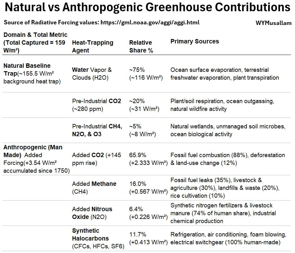
Water vapor has a short atmospheric lifespan, cycling out as rain or snow in about nine days, which means direct human emissions cannot accumulate in the sky.
- However, higher global temperatures expand the atmosphere’s moisture capacity, forcing it to hold more water vapor.
- That extra water vapor then acts as an added thermal blanket, trapping even more heat and doubling the overall warming effect initially triggered by CO2.
Human emissions of CO2 drive nearly two-thirds of all added forcing (man-made or anthropogenic heating) , pushing up global temperatures and forcing the natural water vapor system to trap even more heat.
The other GHGs do their damage as well: You can see their sources in the table.
- Note that methane has a life of about 12 years. It eventually reacts to water and CO2
- The other GHG have even higher lifespans in the atmosphere (14 years to over 1000 years)
Understanding trapped heat shows us what is happening, but tracking the actual carbon shows us why.
Every year, massive amounts of carbon move back and forth naturally:
- plants pull CO2 out of the air through photosynthesis, and
- living things breathe it back out through respiration.
To see how human emissions “disrupt” the natural cycle, we have to look at the actual numbers and run an earth carbon mass balance.
But, before we do that, let’s understand the carbon containing photosynthesis and respiration reactions.
Photosynthesis, Respiration, and Combustion
Photosynthesis
Photosynthesis is a biological process where plants, algae, and cyanobacteria (a certain type of single cell bacteria) use sunlight to convert carbon dioxide CO2 and water H2O into sugar (glucose) and oxygen gas (O2).
Picture: Photosynthesis
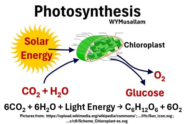
6CO2 + 6H2O + Light Energy → C6H12O6 + 6O2 ; Photosynthesis Equation
- This reaction takes place inside plant cell organelles called chloroplasts, using the pigment chlorophyll to capture light.
- 6 molecules of atmospheric CO2 , 6 molecules of water H2O and absorbed solar energy react to form
- 1 molecule of glucose (C6H12O6 ), which the plant uses as structural biomass or stores for cellular energy,
- and 6 molecules of oxygen (O2 ) released into the atmosphere.
In terms of global carbon mass balance, photosynthesis serves as Earth’s primary biological land sink,
- pulling roughly 130 billion metric tons of carbon out of the atmosphere each year
- before plant and soil respiration return most of it back.
Respiration
Cellular respiration is the biological process where organisms break down glucose using oxygen to release usable energy ATP, producing carbon dioxide CO2 and water H2O as byproducts.
Picture: Respiration
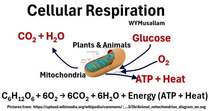
C6H12O6 + 6O2 → 6CO2+ 6H2O+ Energy (ATP + Heat); Respiration Equation
- This reaction takes place inside the cytoplasm and mitochondria of cells across plants, animals, fungi, and microbes.
- 1 molecule of glucose C6H12O6 and 6 molecules of oxygen O2 produces
- 6 molecules of carbon dioxide CO2 , 6 molecules of water H2O , and chemical energy (ATP) to power living cells.
In terms of the global carbon mass balance, respiration is the exact biological reverse of photosynthesis.
- In the carbon balance, it serves as the primary natural emission source on land.
- Autotrophic Respiration (Plants): Plants use about 50% of the carbon they absorb through photosynthesis to fuel their own living functions, venting ~65 billion metric tons of carbon (GtC) back into the sky per year.
- Heterotrophic Respiration (Animals, Fungi & Soil Microbes): Soil microbes, fungi, and animals consume organic plant matter and decay, venting the remaining ~65 GtC per year.
Together, plant and soil respiration return roughly 130 GtC back to the atmosphere annually, creating a balanced biological carbon loop with terrestrial photosynthesis.
Photosynthesis And Respiration Balance Each Other
Photosynthesis and cellular respiration are two halves of the exact same biological loop.
Because the chemical outputs of one process serve as the direct inputs for the other, nature maintains a continuous, self-balancing carbon cycle across the Earth.
Picture: Photosynthesis and Cellular Respiration Are Parts of the Same Natural Loop
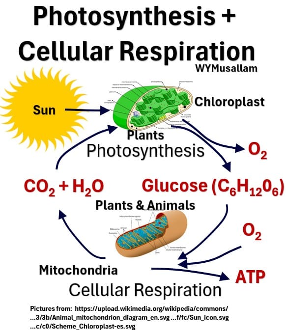
Photosynthesis and cellular respiration form a closed biological loop where the chemical outputs of one process serve directly as the starting inputs for the other.
During photosynthesis, chloroplasts capture light energy to convert carbon dioxide and water into oxygen and glucose.
In turn, mitochondria consume that oxygen and glucose through cellular respiration to yield usable cellular energy (ATP), releasing carbon dioxide and water back into the ecosystem to restart the cycle.
Adenosine triphosphate (ATP) acts as the primary energy currency for all living cells.
Picture – ATP
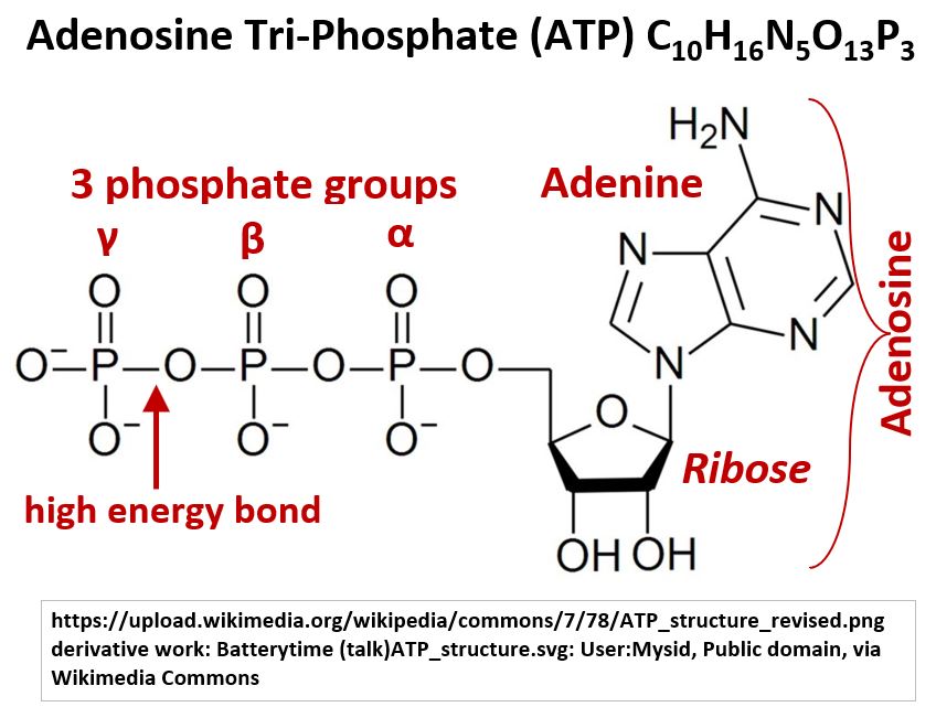
- It stores chemical energy derived from nutrient breakdown within the bonds connecting its three phosphate groups.
- When a cell needs power for vital functions like muscle contraction, nerve signaling, or molecule synthesis, it cleaves the outermost phosphate group, releasing usable energy and leaving behind adenosine diphosphate (ADP).
- Cells then continuously recycle ADP back into ATP to maintain a steady energy supply.
- Read my post on ATP (Adenosine Triphosphate) to learn more about it.
Combustion and Respiration
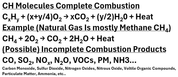
Recall from the “Combustion” section of this article, that the complete combustion of a hydrocarbon CxHy is:
CxHy + (x+y/4)O2 → xCO2 + (y/2)H2O+ Heat : CH Complete Combustion Equation
We showed examples of the equation for the combustion of methane (the major natural gas molecular component) or benzene (a molecular component of gasoline).
Remember that in reality we don’t achieve complete combustion so there will always be incomplete combustion products like CO, SO2, NOx, N2O, VOCs, PM, NH3 and others.
Combustion of a CH Hydrocarbon
Glucose Combustion
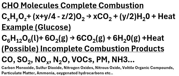
Glucose can also be burned (combusted). Glucose is a hydrocarbon that contains oxygen and it undergoes (ideal) complete combustion according to the equation:
CxHyOz + (x+y/4 – z/2)O2 → xCO2 + (y/2)H2O + Heat : CHO Complete Combustion Equation
C6H12O6 + 6O2 → 6CO2 + 6H2O + Heat : Glucose Complete Combustion Equation
Combustion of an oxygenated Hydrocarbon CHO
Glucose Combustion
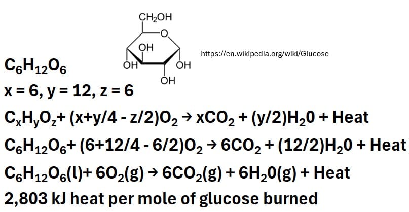
Do you notice something interesting here? The reaction equations for glucose combustion and respiration look almost exactly the same.
- C6H12O6 + 6O2 → 6CO2 + 6H2O + Energy (ATP + Heat); Respiration Equation
- C6H12O6 + 6O2 → 6CO2 + 6H2O + Heat : Glucose Complete Combustion Equation
While both processes share the same net chemical equation, they differ fundamentally in control and energy capture.
- Glucose combustion is an uncontrolled, high-temperature reaction that releases energy all at once as heat and light.
- Cellular respiration is a controlled, multi-step biological process occurring at physiological temperatures that releases energy incrementally to efficiently trap it as ATP.
Photosynthesis, Respiration, Combustion – Putting it all together
The picture below illustrates how atmospheric carbon dioxide and water cycle through biological and industrial pathways via three core chemical processes: Photosynthesis, Respiration, and Fossil fuel Combustion.
Picture: Photosynthesis; Respiration; Combustion
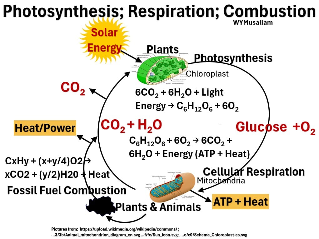
- Photosynthesis: Plants capture solar energy within chloroplasts to fix carbon dioxide and water into oxygen and glucose.
- Cellular Respiration: Plants and animals utilize mitochondria to consume glucose and oxygen, releasing carbon dioxide and water while generating metabolic energy (ATP) and heat.
- Fossil Fuel Combustion: Burning organic fuels reacts with oxygen to produce usable heat and power, adding further carbon dioxide and water into the central reservoir.
While this diagram clearly highlights the chemical alignment between living organisms, solar input, and industrial power generation, it provides only a partial view of the global system.
To appreciate and fully understand the impact of fossil fuel contributions to global warming, we’ll need to incorporate the above into a complete global carbon (CO2 and GHG equivalents) mass (material) balance.
Earth’s Average Carbon Balance
References
- Global Carbon Project. (2026). Supplemental data of Global Carbon Budget 2025 (Version 1.0) [Data set]. Global Carbon Project. https://doi.org/10.18160/gcp-2025
- Global Carbon Budget 2025 Pierre Friedlingstein et al. : https://essd.copernicus.org/articles/18/3211/2026/
- Data supplement to 2025 Global Carbon Budget; https://www.icos-cp.eu/impact/science/global-carbon-budget/2025
- Global Carbon Project (GCP): https://www.globalcarbonproject.org/
Consider the simplified picture below of Earth’s CO2 Balance.
Earth CO2 Balance Simplified
Picture: Earth CO2 Balance
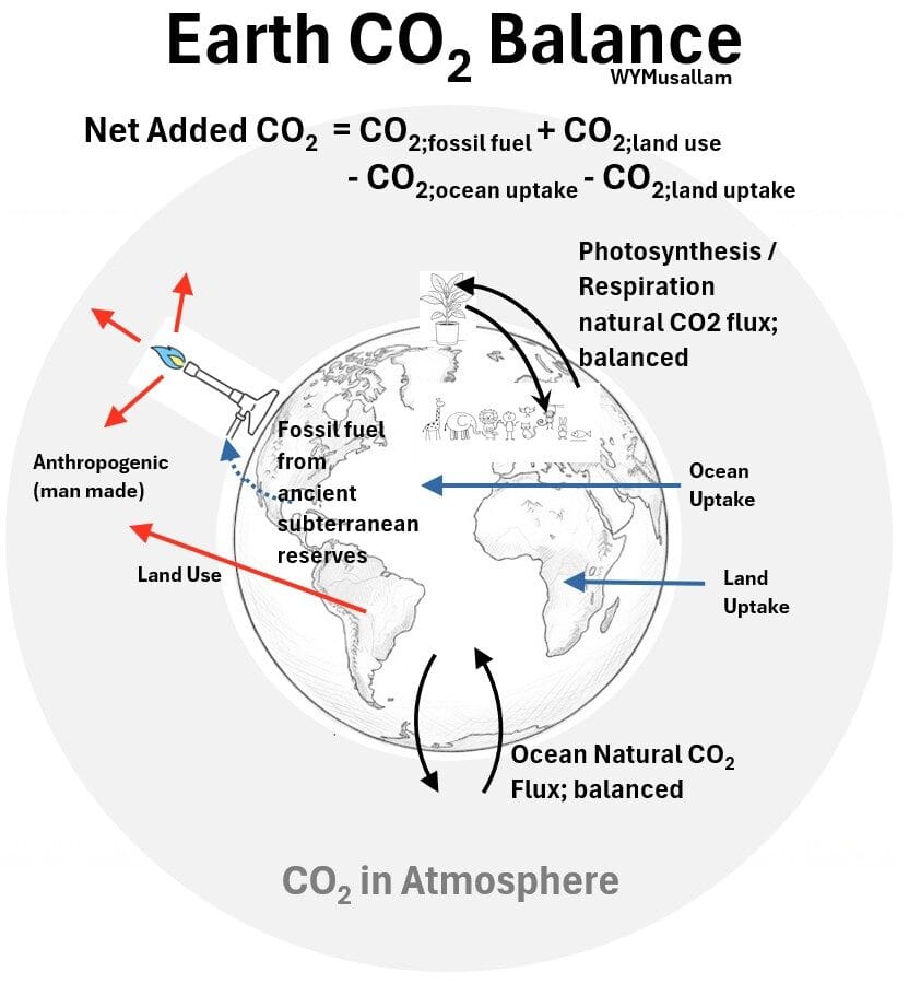
This diagram illustrates the global carbon dioxide CO2 balance (or budget), detailing how human activities alter the natural balance of atmospheric CO2.
Net Added CO2 = CO2;fossil fuel + CO2;land use – CO2;ocean uptake – CO2;land uptake
Anthropogenic Sources (Emissions)
- Fossil Fuel Emissions: CO2 released into the atmosphere by extracting and burning ancient subterranean carbon reserves.
- Land Use: Emissions generated through human land activities such as deforestation, land clearing, and agriculture.
Natural Carbon Sinks (Uptake)
- Ocean Uptake: Atmospheric CO2 absorbed directly by surface ocean waters.
- Land Uptake: Increased CO2 absorbed by terrestrial vegetation and soil systems.
Balanced Natural Cycles
- Photosynthesis / Respiration: Equal bi-directional exchange of CO2 between plant/animal life and the atmosphere.
- Ocean Natural CO2 Flux: Naturally balanced equilibrium of CO2 exchange between the ocean surface and the atmosphere.
Key Points
- The diagram highlights that pre-industrial natural cycles, photosynthesis/respiration on land and air-sea exchange in the ocean, operate as closed, balanced loops with zero net atmospheric accumulation.
- Fossil fuels , are stored in the Earth for millions of years. Burning them introduces “new” active carbon into the surface atmosphere.
- Earth’s land biosphere and oceans (uptakes) act as net absorbers (sinks), soaking up a substantial fraction of human emissions.
- But uptake rates cannot keep pace with total emissions, so the net result is a continuous accumulation of atmospheric CO2
- The diagram distills complex global biogeochemistry into a simple four-term equation: two anthropogenic inputs (fossil fuels, land use) minus two natural sinks (ocean uptake, land uptake).
Earth Carbon Balance – Detailed
Let’s now add some numbers and additional details to describe climate scientists’ latest views of the Earth’s carbon balance.
The following chart is based on information from the Global Carbon Project. (2026). Supplemental data of Global Carbon Budget 2025 (Version 1.0) [Data set].
Picture: Carbon Balance: 2015 – 2024 Average Mass Flows and Carbon Pools
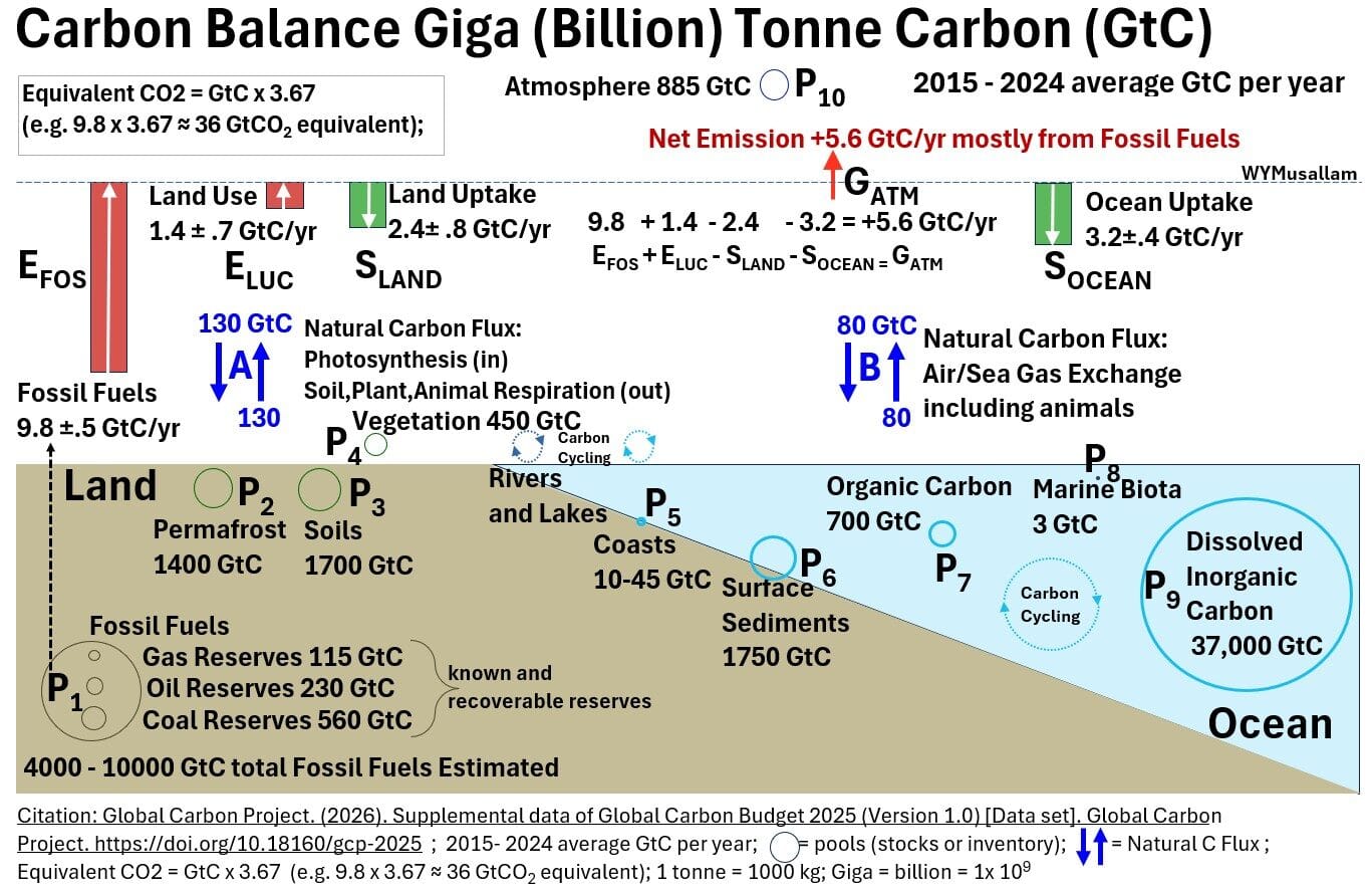
Scope & Conversion Rules
- Definition of GtC: Giga (billion) tonne (metric tonne) Carbon.
- Definition of “Carbon” C: Measures just the elemental carbon mass isolated within various chemical compounds across Earth’s reservoirs; including atmospheric gas (CO2, CH4), biological structures (cellulose, organic matter), ocean minerals (carbonates), and fossil hydrocarbons.
- Exclusions: Excludes the mass of accompanying atoms (such as oxygen in CO2 or hydrogen in hydrocarbons) as well as non-carbon atmospheric constituents (N2, O2, H2O, CFCs).
- C to CO2 Conversion: To convert from C to CO2 , multiply by 3.68 ; where 3.68 is the ratio of the molecular weights of CO2 and C.
Global Carbon Balance Summary (2015–2024 Averages)
1. Anthropogenic Net Budget
Human activities emit 11.2 GtC/yr, while natural sinks reabsorb 5.6 GtC/yr, leaving a net accumulation rate of +5.6 GtC/yr in the atmosphere (GATM):
GATM = EFOS + ELUC – SLAND – SOCEAN
+5.6 GtC/yr = 9.8 + 1.4 – 2.4 – 3.2
Emissions Inputs (+11.2 GtC/yr):
- Fossil Fuels (EFOS): 9.8 ± 0.5 GtC/yr; (combustion of coal, oil, gas).
- Land Use Change (ELUC): 1.4 ± 0.7 GtC/yr; (deforestation, land clearing).
Natural Sinks (-5.6 GtC/yr):
- Ocean Uptake (SOCEAN): 3.2 ± 0.4 GtC/yr; (direct air-sea absorption).
- Land Uptake (SLAND): 2.4 ± 0.8 GtC/yr; (plant growth, soil sequestration).
2. Natural Background Fluxes
In contrast to net anthropogenic additions, background gross exchanges exist in continuous dynamic equilibrium:
- Terrestrial (Land) Exchange: 130 GtC/yr absorbed via photosynthesis and 130 GtC/yr released via respiration.
- Ocean Exchange: 80 GtC/yr absorbed and 80 GtC/yr released across the ocean surface.
3. Carbon Pools / Reservoirs (P1 – P10)
- Atmosphere (P10): 885 GtC ; total stock.
- Ocean System (P6 – P9): 37,000 GtC as dissolved inorganic carbon (P9), 1,750 GtC surface sediments (P6), 700 GtC organic carbon (P7), and 3 GtC marine biota (P8).
- Terrestrial System (P2 – P5): 1,700 GtC soils (P3), 1,400 GtC permafrost (P2), 450 GtC vegetation (P4), and 10 -45 GtC aquatic/coastal zones (P5).
- Geological Reserves (P1): 905 GtC in known recoverable fossil fuels (560 GtC coal, 230 GtC oil, 115 GtC gas) out of an estimated 4,000 -10,000 GtC total reserves.
Picture: Global Carbon Cycle Balance Overall
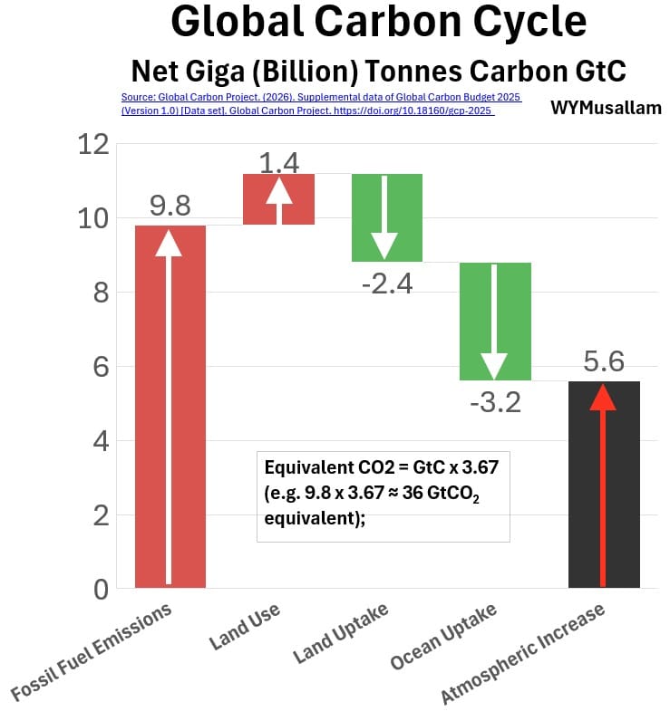
Key Takeaways
- Natural exchanges (130 GtC/yr terrestrial, 80 GtC/yr oceanic) are massive, but they operate as balanced closed loops where “In”≈”Out” .
- Fossil fuel burning (9.8 GtC/yr ) is a one-way injection from ancient subterranean storage (P1) into the surface system.
- By mass balance (dM/dt=”Inputs”-“Outputs” ), any unbalanced input results in continuous mass accumulation dMATM /dt = +5.6 GtC/yr .
- Sinks (uptakes) provide only a 50% Buffer: Ocean (3.2 GtC/yr ) and land (2.4 GtC/yr ) uptake reabsorb roughly half of total human emissions (11.2 GtC/yr ).
- While these natural sinks mitigate the rate of increase, they lack the capacity to clear the full surplus.
- The atmosphere holds a relatively small inventory (885 GtC ) compared to deep oceans (37,000 GtC ) or soils (1,700 GtC ).
- Adding a net +5.6 GtC annually to an 885 GtC tank creates a rapid relative concentration shift (~0.63% growth per year).
- Total estimated fossil reserves (4,000-10,000 GtC ) are roughly 5 to 11 times larger than the entire atmospheric carbon pool (885 GtC ), demonstrating that extracting even a fraction of remaining deposits would drastically reshape atmospheric composition.
Global Warming Data and Evidence
References
- https://gml.noaa.gov/aggi/
- https://www.climate.gov/news-features/climate-qa/what-evidence-exists-earth-warming-and-humans-are-main-cause
- https://science.nasa.gov/climate-change/evidence/
- https://science.nasa.gov/earth/explore/earth-indicators/global-temperature/
- https://www.climate.gov/news-features/understanding-climate/climate-change-global-temperature
- https://www.climate.gov/climatedashboard
Global Warming Recap
So, we’ve learned that the Earth’s greenhouse gas laden atmosphere absorbs and re-emits radiation from the earth with only a portion of it escaping to earth.
Consider the simplified drawing below.
Picture: Global “Greenhouse” Warming
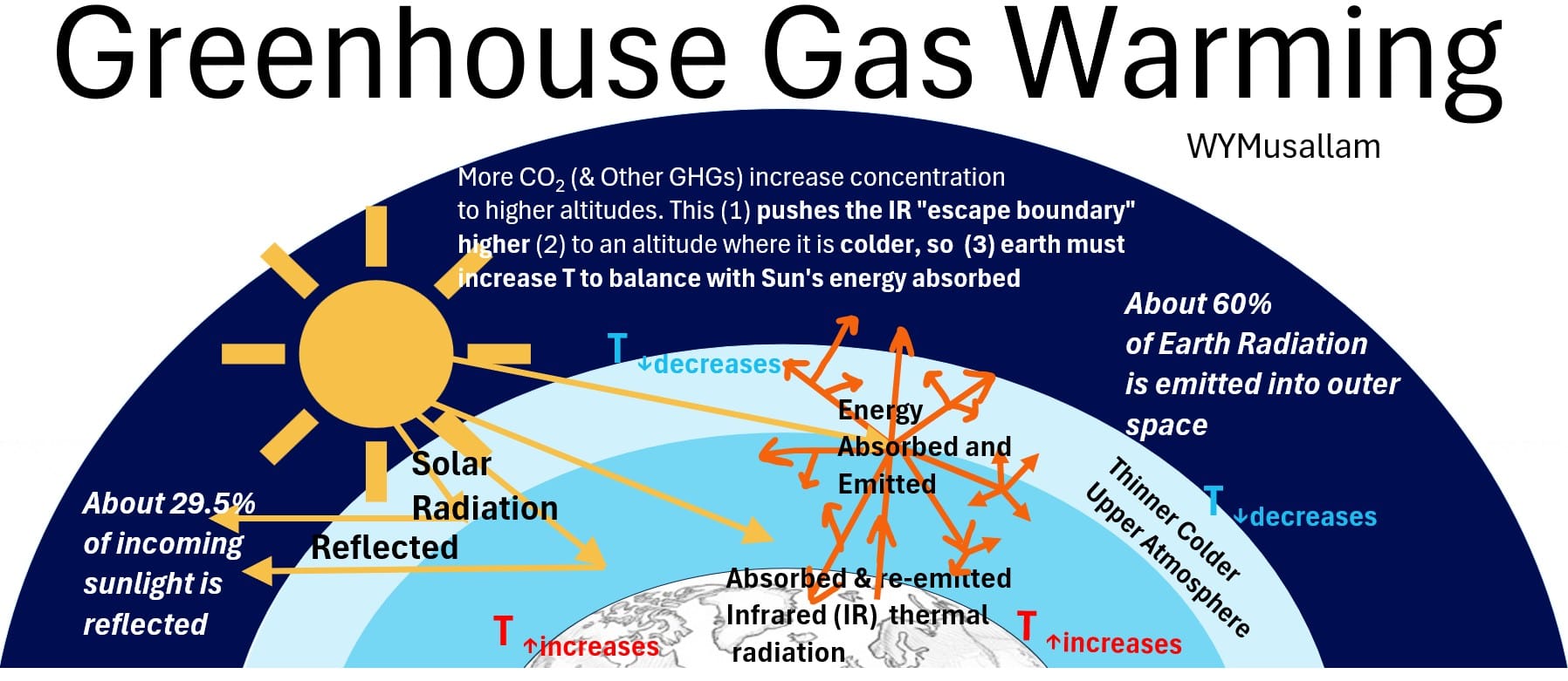
This diagram breaks down the radiative physics behind global warming against a layered atmospheric backdrop.
- The sun projects solar radiation toward Earth, with yellow arrows indicating that roughly 29.5% of incoming sunlight is reflected straight back into space due to albedo.
- Energy from the sun is also directly absorbed by GHGs in the atmosphere.
- The Earth absorbs the remaining energy and re-emits it upward as thermal radiation, represented by a branching network of orange arrows showing absorbed and re-emitted infrared (IR) energy.
- Approximately 60% of Earth’s thermal radiation eventually escapes into outer space through the thinner, colder upper layers of the atmosphere.
The top section of the image details the specific thermodynamic mechanism driven by greenhouse gases.
- As concentrations of CO2 and other greenhouse gases increase, they extend into higher atmospheric altitudes.
- This pushes the IR “escape boundary” upward into colder air layers;
- because less heat radiates into space at these lower temperatures, the Earth’s surface and lower atmosphere must experience a temperature (T) increase to balance the total solar energy absorbed.
CO2 (mainly) is the cause of global warming.
- It’s sometimes called the “radiative forcing agent”.
- It’s the primary driver; the causal factor.
The core climate indicator that reflects this warming is of course temperature and this rise in temperature affects the earth in various ways
Let’s explore the CO2 and Temperature data that scientists collect and track and then provide examples of what these cause on earth (the evidence).
Global Warming Bathtub Analogy
Global warming is fundamentally an energy balance problem best understood as a bathtub whose drain is slowly being clogged, forcing the water level to rise until pressure restores the balance.
Consider the bathtub drawing below where we have a flow of water coming in through the faucet and flowing out through the drain.
Picture: Bathtub Analogy to Global Warming
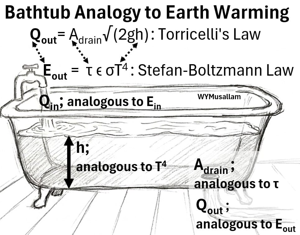
There are two equations at play here; Torricelli’s Law
Qout = Adrain√(2gh)
where
- Qout : Outflow rate (volumetric fluid discharge)
- Adrain: Cross-sectional area of the drain
- g: Acceleration due to gravity
- h: Height of the water column (hydrostatic head)
and the Stefan-Boltzmann Equation
Eout = τεσT4
where
- Eout: Outgoing longwave thermal radiation flux
- τ: Atmospheric transmissivity (we said this was about 60%). Transmissivity describes the transmission efficiency of an intervening medium (the atmosphere).
- ε: Surface emissivity of the Earth (we assume 1)
- σ: Stefan-Boltzmann constant
- T: Absolute surface temperature
Picture: Bathtub Analogy to Global Warming – Table
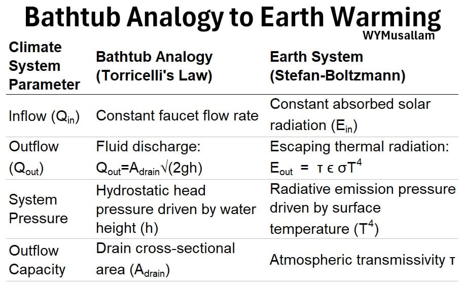
The analogy of the draining bathtub to a warming Earth goes as follows:
Step_1: Steady-State Equilibrium (Temperature and Height analogy)
- Bathtub: Water enters at Qin and exits through drain area Adrain at rate Qout = Adrain √(2gh).
- Inflow equals outflow keeping water level h completely stable.
- Earth: Solar energy enters at Ein and exits through atmospheric transmissivity τ at rate Eout = τεσT4.
- Transmissivity describes the transmission efficiency of an intervening medium (the atmosphere).
- Energy input equals radiation output, keeping surface temperature T completely stable.
Step_2: Restricting Outflow Capacity (Transmittivity τ and Adrain analogy )
- Bathtub: A partial clog reduces the drain area (Adrain ↓). With less area to exit, Qout drops below Qin.
- Earth: Greenhouse gases accumulate, lowering atmospheric transmissivity ( τ ↓ ).
- With less infrared light passing through directly to space, Eout drops below Ein.
Step_3: Accumulating Mass and Energy (Qin > Qout; Ein > Eout )
- Bathtub: Because Qin > Qout , water has nowhere to go and begins accumulating in the tub (h starts rising ↑).
- Earth: Because Ein > Eout , thermal energy has nowhere to go and begins accumulating in the climate system.
Step_4: Building Pressure to Force Outflow (h ↑ ; T ↑)
- Bathtub: Accumulated water causes water height h to rise.
- Under Torricelli’s Law, a higher water level h creates greater hydrostatic head pressure, pushing water through the constricted drain Adrain faster.
- Earth: Accumulated heat causes surface temperature T to rise.
- Under the Stefan-Boltzmann Law, a higher temperature T creates stronger thermal emission “pressure” (T4 ↑ ), pushing infrared energy through the “restricted” atmosphere τ faster.
Step_5: Re-establishing Equilibrium at a Hotter Baseline (h2 > h1 ; T2 > T1)
- Bathtub: The water level stops rising once h reaches a high enough level (h2) where hydrostatic pressure forces Qout to match Qin again: Qout = Adrain2√(2gh2)
- Earth: Temperature stops rising once T reaches a high enough level (T2) where thermal pressure T4 forces Eout to match Ein again: Qin = τ2 εσT24
The temperature increase from T1 to T2 is global warming; the exact physical equivalent of a bathtub needing a higher water level (h2) to maintain flow balance through a clogged drain.
CO2 Data
How and Where is it Measured? Is it Accurate?
Atmospheric carbon dioxide CO2 is continuously monitored across a global network of remote, high-altitude observatories (for example, Hawaii’s Mauna Loa Observatory at 3,400 meters elevation) using optical spectroscopy instruments that measure the exact amount of infrared light absorbed by clean, dry air samples.
- Relying on Mauna Loa’s record alone is fully indicative of planetary climate trends because CO2 persists in the atmosphere for centuries, giving global winds ample time to thoroughly mix the gas across the globe within a single year.
- Positioned far from major industrial pollution, Mauna Loa samples pristine, well-mixed air from the upper troposphere that stays within 1 to 2 parts per million (less than 0.5%) of the global ocean-and-land average, while rigorous automated filtering routinely strips out any localized volcanic or plant emissions.
- As a result, Mauna Loa’s data curve functions as a very precise proxy for the entire planet, capturing both the Earth’s natural seasonal biosphere cycles and its long-term atmospheric trajectory.
Historical CO2 Trends
The graph below displays the Keeling Curve ; the direct measurement of atmospheric carbon dioxide taken at Hawaii’s Mauna Loa Observatory since 1958.
Graph: Historical CO2 at Mauna Loa Observatory
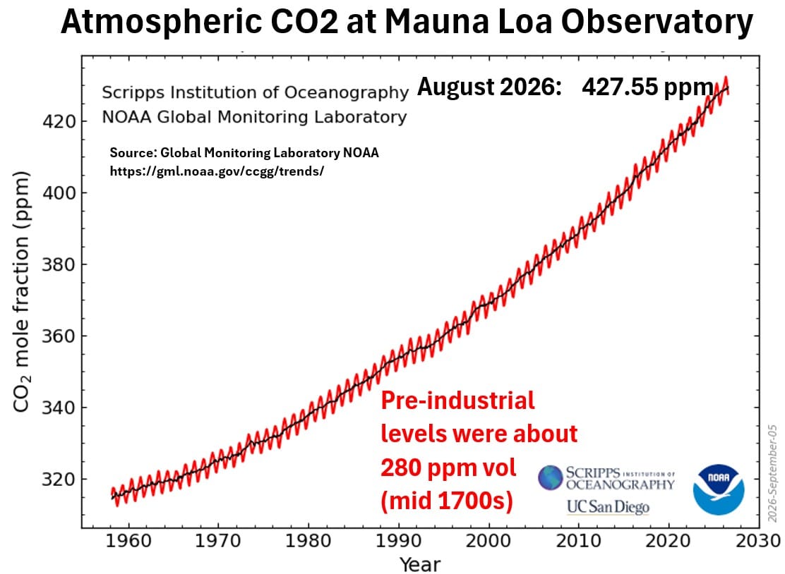
- The “Seasonal Sawtooth”: The fine red zig-zag captures Earth’s seasonal respiration. CO2 levels dip each spring and summer as vast Northern Hemisphere forests photosynthesize and draw down carbon, then peak in winter and early spring as vegetation decays and releases it back.
- Accelerating Velocity: The trend line isn’t just going up—it is steepening. In the 1960s, atmospheric CO2 increased by roughly 0.9 ppm per year, whereas the current growth rate routinely exceeds 2.0 to 2.5 ppm per year.
- Major Baseline Shift: Reaching 427.55 ppm in August 2026 represents a >52% increase over the ~280 ppm pre-industrial baseline, pushing atmospheric concentrations into territory unprecedented in human history.
- Institutional Benchmark: Maintained through combined data from the Scripps Institution of Oceanography and NOAA, this record serves as the global baseline for tracking human-driven greenhouse gas accumulation.
The NASA graph below tracks atmospheric carbon dioxide CO2 levels over the past 800,000 years, contrasting historical natural cycles with modern concentrations.
Graph: Historical CO2 Levels over the past 800,000 years
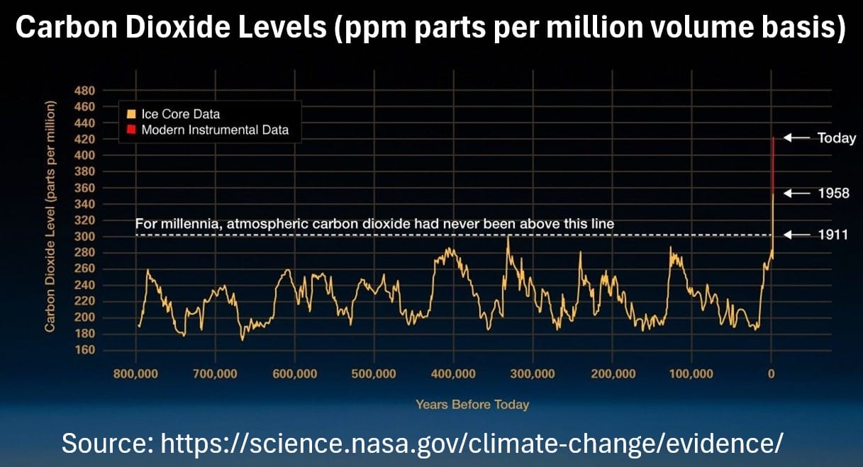
- Data Sources: Ancient ice core data (yellow) with direct modern instrumental measurements (red) are used to measure CO2.
- Historical Baseline: Shows natural fluctuations bounded between about 180 ppm and 300 ppm across eight glacial/interglacial cycles over 800,000 years.
- The 300 ppm Threshold: Features a dashed reference line at 300 ppm to highlight that atmospheric CO2 never exceeded this level for millennia prior to the 20th century.
- Modern Surge: Demonstrates a steep, nearly vertical rise beginning around 1911, climbing past 315 ppm in 1958 to over 420 ppm today
Temperature
How/Where is Temperature measured?
Global surface temperature is measured through a worldwide network of thousands of land weather stations, ocean buoys, research ships, and satellite radiometers.
- To standardize these diverse inputs, scientists convert raw readings into temperature anomalies (deviations from a long-term local baseline) which neutralizes geographic and elevation differences.
These measurements are exceptionally reliable:
- automated processing algorithms rigorously correct for non-climatic biases, such as station relocations, changing measurement times, or urban heat island effects.
- Independent international research groups (including NASA, NOAA, the European Union’s Copernicus, and Berkeley Earth) apply different processing methodologies to the raw data and arrive at virtually identical global warming trends within fractions of a degree
NOAA Temperature Departure (Anomaly) Data
The below NOAA anomaly (temperature departure) chart shows the global surface temperature outcome of rising atmospheric CO2 levels.
Graph: NOAA Anomaly (Temperature Departure) Data
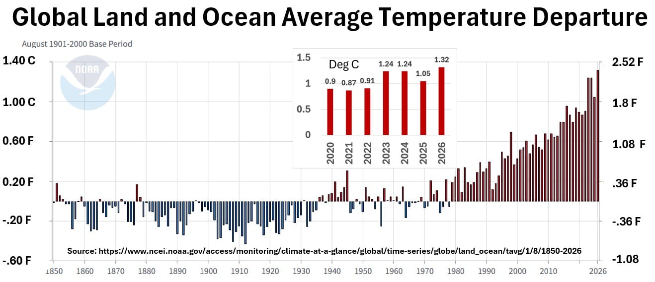
- A temperature departure is calculated by subtracting a location’s long-term historical average for a given month from its actual recorded temperature.
- These local differences are then area-weighted and averaged across the globe to produce the overall temperature anomaly.
- The Blue-to-Red Shift: Visualizes a stark regime change from a cooler 19th and early-20th century (dominated by blue bars below the 1901–2000 average) to an unbroken, multi-decade sequence of above-average temperatures beginning in the late 1970s.
- Steepening Modern Spike: The last decade (2015–2026) displays an unprecedented cluster of extreme August anomalies, with temperatures spiking sharply to nearly +1.3°C (+2.3°F) above the 20th-century baseline.
- Baseline Nuance: Because NOAA uses the 20th-century average (1901–2000) for its zero reference line, total warming compared to true pre-industrial levels (1850–1900) is actually an additional ~0.2°C to 0.3°C higher than depicted here.
- Coupled Warming: By integrating both land and sea surface data, the chart highlights that thermal inertia across global oceans is being systematically overcome alongside land surface warming.
But The Temperature Change is So Small. How could it possibly do any damage?
https://www.climate.gov/news-features/understanding-climate/climate-change-global-temperature
While NOAA’s chart displays a 1.32°C anomaly based on a 20th-century average (1901–2000), adjusting to the cooler pre-industrial baseline (1850–1900) used by the IPCC brings total warming right to the standard 1.5°C benchmark.
But so What? Since pre-industrial times our Earth’s temperature has risen 1.5 C but an average person in the United States experiences an outdoor annual temperature range of 30°F to 90°F (-1°C to 32°C) across changing seasons.
This amount sounds trivial because in most human contexts, we experience a much wider range of temperature and do just fine.
- Equating short-term local weather swings with the global climate baseline is the central disconnect in climate communication.
- We need to come back to our energy balance to understand this.
Recall our energy balance (see picture below) from the “Earth Average Energy Balance” section.
Picture: Earth Average Energy Balance (2015 – 2023)
Today (latest data at least) earth emits about 398 Watts per square meter (W/m²) emitted by the earth and the Stefan-Boltzmann equation (see “Stefan-Boltzmann Equation” section) tells us this is equivalent to a blackbody radiator at 16.3 C (Adjusted for Latent and Sensible Heat Cooling it’s more like 15 C).
- E = τεσT4 where σ = Stefan-Boltzmann constant = 5.670 × 10⁻⁸ W/m2/K4, T = temperature in Kelvin (C + 273.15 = K), τ = transmissivity = 60% , and ε = emissivity as a percent efficiency factor assumed to be 100%
- For E = 398, T = 16.3 C (See “Average Earth Energy Balance” section)
- Adjusted for latent and sensible heat cooling effects, T actual is more like 15 C (we could have assumed τ = 62% to get this result using the equation)
The pre-industrial baseline for radiation emitted from earth is about 390 W/m².
So in terms of the Earth’s energy balance, driving a 1.3°C total surface warming requires trapping an extra 8 W/m² ( 398 – 390 = 8 W/m²) of thermal radiation continuously across every square meter of Earth.
- That accumulated surplus equals roughly 4,000 Terawatts of excess power; over 200 times the energy output of all human civilization combined, or
- physically equivalent to leaving an 80-watt heat lamp running non-stop over every single 10-by-10-foot patch of land and ocean on the planet.
That vast energy surplus doesn’t sit idle.
Looking at the energy diagram we have 82 W/m² of Latent Heat flow, much of this extra heat acts as a massive contributor to global evaporation, forcing oceans to boil off water vapor at unprecedented rates.
This supercharges storm systems, dries out soils into mega-droughts, and bakes the oceans.
A 1.5C warming shift is not a mild change in weather; it is the signature of trillions of watts of raw energy permanently altering the Earth system.
A useful analogy is the core temperature of the human body.
- A healthy human maintains a tightly regulated core temperature near 98.6°F (37°C).
- Similarly, Earth’s climate relies on a delicate energy balance between incoming solar radiation and outgoing heat to maintain a stable planetary baseline.
- External Fluctuation vs. Core Shift: You can comfortably walk from a 70°F air-conditioned room into a 95°F afternoon because your body actively regulates its core.
- However, if your internal core temperature rises by just 2°F to 100.6°F, you have a fever.
- Earth easily handles 20°F local daily weather swings, but a 2°F rise in its total global average represents a planetary “fever”.
- Cascading Symptoms: A fever isn’t just “feeling warmer”; it triggers systemic stress, inflammation, and organ strain.
- Likewise, a small upward shift in global baseline temperature triggers cascading symptoms across planetary systems: jet stream destabilization, ocean heatwaves, and accelerated ice sheet collapse
Average versus Extremes
Another way to think of an increase in average temperature is to think of what that means regarding the extremes.
The image below shows two “bell” curves mapping out daily temperatures (normal probability distributions).
Picture: Global Warming Shift Shown on Two Normal Distribution Curves
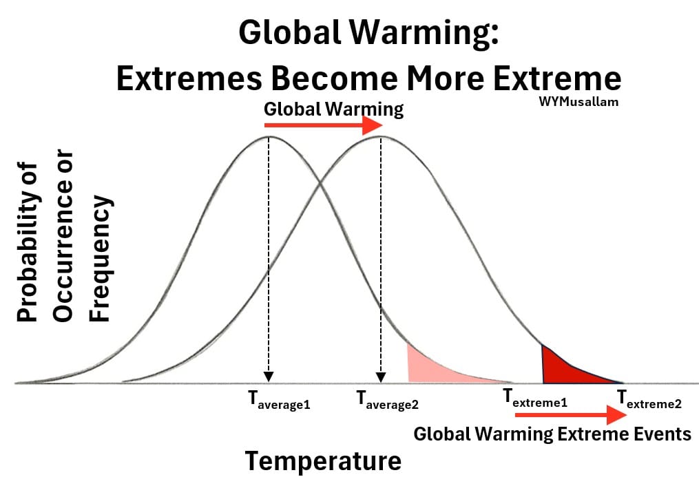
The second curve is identical to the first, just slid to the right, and represents a hypothetical increase in average global temperatures.
When thinking about global warming, the average temperature isn’t what matters—it’s the extreme events.
- A few extra degrees on a normal day is barely noticeable, but those same extra degrees added to an already dangerous heatwave turn it into a disaster.
Evidence
I encourage you to read more about each of these using the links provided below
References
- https://science.nasa.gov/climate-change/evidence/ ; Google Gemini
- https://www.climate.gov/climatedashboard
- Google Gemini
Beyond rising atmospheric CO2 levels and global surface temperatures, climate scientists track key empirical indicators across the ocean, ice sheets, and biosphere to measure accelerating planetary warming:
Cryosphere Breakdown (Ice & Snow)
- Shrinking Ice Sheets: Satellite observations hosted on NASA’s Sea Level Change Portal show Greenland losing ~260 billion metric tons of ice per year and Antarctica losing ~100 billion metric tons annually, directly driving sea level rise.
- Glacial Retreat: The US Geological Survey (USGS) documents accelerated mountain glacier loss worldwide, which alters regional hydrology and threatens freshwater supplies.
- Permafrost Thaw & Sea Ice Decline: Reports from the US EPA Climate Change Indicators track steady declines in Arctic sea ice extent along with rising permafrost ground temperatures across northern latitudes, which threatens northern infrastructure and releases trapped methane.
Ocean Heating & Chemical Shifts
- Record Ocean Heat Content: Data from NOAA Climate.gov indicate oceans store over 90% of the excess heat trapped in Earth’s climate system, fueling severe marine heatwaves and widespread coral bleaching.
- Accelerating Sea Level Rise: Measurements on NASA Earth’s Sea Level Portal record over 100 millimeters of global sea height variation since satellite tracking began in 1993, driven by thermal expansion of warming seawater and melting land ice.
- Ocean Acidification: Monitoring by the NOAA Ocean Acidification Program tracks declining surface ocean pH levels as seawater absorbs excess atmospheric carbon dioxide, disrupting marine food webs and calcifying organisms.
Atmospheric & Extremes Indicators
- Accelerating Global Surface Temperatures: Historical analysis from NOAA National Centers for Environmental Information shows global warming has accelerated to more than three times its 1850–1975 rate over recent decades, making the past decade the warmest on record.
- Extreme Weather Frequency: The US EPA Climate Indicators Dashboard details measurable increases in heatwave frequency, heavy precipitation events, prolonged mega-droughts, and lengthening wildfire seasons.
Appendix 4 – Area Under the Curve for a Linear , Log2 Spectral Radiation Chart
Graph: Linear log2 Graph of Sun and Earth Radiation Curves
I used excel to plot the data above using Planck’s law (wavelength form for radiant exitance/emittance) and a graphing strategy described in the following reference
The areas under these curves for the sun and earth are the total E/m2 they possess over the full wavelength range.
To prove why the area under the curve equals the total power per square meter (SI units: W/m2), we can set up the standard geometric area integral for the axes in the graph above.
In any Cartesian plot, the geometric area under a curve is calculated by integrating the Y-axis values with respect to the position on the X-axis:
- 1. Area= ∫ YdX i.e. the sum of the infinitesimal areas defined by Y dx.
- 2. Area = ∫ Edλ ; we know this area = total Emittance in power per square meter (SI units: W/m2)
Step_1: Define Your Axis Variables
- 3. Y-axis value: Y = Eλln(2) where ln is the natural log
- 4. X-axis value: X = log2λ where log2 is logarithm base 2
We can express 4. as
- 5. dX = dlog2λ
Step_2: Set Up the Area Integral
Substitute equations 5 and 3 into equation 1
- 6. Area = ∫ Eλln(2)d(log2λ)
Step_3: Convert the Logarithmic Differential
From calculus, the change-of-base rule for logarithms tells us that:
- 7. d(log2λ) = (1/ln(2))(dλ/λ)
Step_4: Substitute and Simplify
Now, substitute that conversion back into equation 6.
- 8. Area = ∫Eλln(2)(1/ln(2))(dλ/λ)
The ln(2) and λ terms cancel out of equation 8 and we end up with
- 9. Area = ∫Edλ = Equation 2 = Total Emittance in W/m2
Conclusion
By definition, the integral of spectral emittance over all wavelengths Area = ∫ Edλ is the total emittance measured in W/m2
This proves that even though the X-axis is stretched logarithmically and the Y-axis is multiplied by λ ln(2), the physical area under the curve on the chart is mathematically identical to the standard linear area under the raw spectrum.
Return to “Earth and Sun Radiation Spectra Compared” Section
Appendix 5 – Planck’s Law, Derivation of Stefan-Boltzmann Law and Wien’s Displacement Law, and Definitions of Spectral Radiance and Spectral Radiant Exitance (Emittance).
Sources/References:
Planck’s Law
Planck’s Law describes how much electromagnetic radiation a blackbody emits.
- It describes the spectral distribution of electromagnetic radiation emitted by a blackbody in thermal equilibrium at a specific temperature.
- It mathematically shows that hotter objects emit more overall energy and peak at shorter, bluer wavelengths by establishing that energy is radiated in discrete packets called quanta.
Max Planck presented the equation for Planck’s Law in October and December of 1900 to the German Physical Society.
Planck’s Law can be expressed in terms of Spectral Radiance (its foundational form) or Spectral Radiant Exitance (or Emittance).
So before we discuss the Planck’s law equation , let’s get clear on what radiance vs exitance/emittance means.
Spectral Radiance
Spectral radiance measures the radiant flux (power) emitted by a surface
- per unit projected area (SI units of m2)
- per unit solid angle (sr = steradian)
- per unit frequency nu (in Hz), or wavelength λ (in meters) interval
We snuck in a strange term called the steradian. Let’s describe it next.
What is a Steradian?
- If you project a beam of light from the center onto the inside wall of that sphere, it will trace out a circular patch.
- If you expand that beam until the illuminated patch on the wall covers an area of exactly 1 square meter, the angle of that light cone is exactly 1 steradian.
- If the patch is a circle, then the cone angular spread is defined by the steradian i.e. the steradian is an angular spread factor
- For example, 1 steradian defines a cone whose half and full apex angular spreads are 32.74 and 65.5 degrees respectively
Picture: Steradian Defined
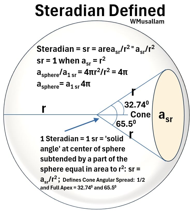
Spectral Radiant Exitance (or Emittance)
Spectral radiant exitance (or emittance) measures the radiant flux (power) emitted by a surface
- per unit area (SI units of m2)
- per unit frequency nu (in Hz) (or wavelength lambda in meters) interval.
Notice that per unit solid angle is left out of the exitance definition.
- Because exitance integrates all directions across the entire hemisphere,
- the angular component and the directional projection are summed away,
- leaving it as total power per standard surface area per spectral slice.
Wavelength and Frequency Forms of Planck’s Law
Planck’s_law is written in two primary ways depending on how you choose to represent the light spectrum: by wavelength or by frequency.
Planck’s Law: Wavelength Form; Spectral Radiance
Lλ(λ, T) = (2hc2) / (λ5 * (e(hc / λkBT) – 1))
SI Units: W/{(sr)(m2)(m)}
Planck’s Law: Frequency Form; Spectral Radiance
Lν(ν, T) = (2hν3) / (c2 * (e(hν / kBT) – 1))
The SI Units: W/{(sr)(m2)(Hz)} = W/{(sr)(m2)(s-1)}
Variables and Constants:
- Lλ = Spectral radiance as a function of wavelength
- Lν = Spectral radiance as a function of frequency
- λ = Wavelength of the light (measured in meters)
- ν = Frequency of the light (measured in Hertz)
- T = Absolute temperature (measured in Kelvin)
- e = The natural logarithm base (≈ 2.718)
- h (Planck’s constant) = 6.626 × 10⁻³⁴ J · s
- c (Speed of light) = 3.00 × 10⁸ m/s
- kB (Boltzmann’s constant) = 1.381 × 10⁻²³ J/K
Planck’s_Law (Spectral Radiant Exitance or Emittance = M)
Planck’s Law: Wavelength Form; Spectral Exitance/Emittance
Mλ(λ, T) = π · Lλ = (2πhc2) / (λ5* (e(hc / λkBT)– 1))
Planck’s Law: Frequency Form; Spectral Exitance/Emittance
Mν(ν, T) = π · Lν = (2πhν3) /(c2 * (e(hν / kBT) – 1)– 1))
Core Assumptions That Must Hold True for the Exitance/Emittance equations:
- For this simple conversion to work, you must assume the emitting surface is an ideal Lambertian surface (a perfectly diffuse radiator).
- This means the surface radiates energy equally in all directions. Because the directional terms drop out of the complex spherical trigonometry integrals, the entire double-integration over a 3D hemisphere collapses mathematically into a single multiplier of π.
Recap:
- Radiance (L or B) measures the power traveling in a specific direction.
- Its unit contains sr (steradians), which accounts for that directional cone of vision.
- Radiant Exitance (M) measures the total power leaving the surface in all upward directions combined.
- Because you have integrated across the entire hemisphere, the directional component is gone.
- The unit sr disappears completely, changing the SI unit
- from Watts per steradian per meter squared per meter of wavelength: W/{(sr)(m2)(m)}
- to simply Watts per meter squared per meter of wavelength: W/{(m2)(m)}
Derivation of the Stefan-Boltzmann Law
1. The Total Integral
2. Calculus Substitution
- To solve this, we use a u-substitution trick.
- Let a new variable x equal the exponent: x = (hc) / (λkBT)
- By substituting x and its derivative back into the integral, we pull all the constant terms outside of the calculus boundaries.
E = [ (2πkB4T4) / (h3c2) ] * ∫0∞ (x3 / (ex – 1)) dx
3. Final Steps
- The remaining definitive integral is a classic mathematical form related to the Riemann zeta function, which evaluates exactly to (π4 / 15).
- Substituting this back into the equation yields:
- E = [ (2π5kB4) / (15h3c2) ] · T4
- Every term inside those brackets is a constant.
- Scientists bundle them together into a single value known as the Stefan-Boltzmann constant (σ):
- σ = (2π5kB4) / (15h3c2) = 5.670 × 10⁻⁸ W · m-2 · K-4
This leaves us with:
E = σT4 : Stefan-Boltzmann Equation
where
- σ = Stefan-Boltzmann constant = 5.670 × 10⁻⁸ W/m2/K4
- T = temperature in Kelvin (C + 273.15 = K)
- We typically express it as E = εσT4 where ε = emissivity as a percent efficiency factor is assumed 100%
- You will also see this expressed as E = τεσT4
- where we add the variable τ representing transmissivity which describes the transmission efficiency of an intervening medium (the atmosphere).
Derivation of Wien’s Displacement Law
1. Differentiating
- d(Mλ) / dλ = 0
- Applying the product and chain rules to the Planck exitance equation removes the leading constants and sets up a transcendental equation.
- Using our previous substitution where x = (hc) / (λkBT), the relationship simplifies directly to: 5 – x = 5e-x
2. Numerical Solving
- This specific equation cannot be broken down using basic algebra; it must be solved numerically.
- Finding the root for x yields: x ≈ 4.96511
3. Isolating the Peak
- Now we swap our original variables back in place of x:
- (hc) / (λmaxkBT) = 4.96511
- Isolating the product of the peak wavelength (λmax) and the temperature (T) on one side gives us:
- λmax · T = (hc) / (4.96511 · kB)
4. Finding the Constant
- Calculating the value of the constants on the right side:
- b = (6.626 × 10-34 * 3.00 × 108) / (4.96511 * 1.381 × 10-23) ≈ 2.898 × 10⁻³ m · K
λmaxT = b : Wien’s Displacement Law
where
- b is Wien’s displacement constant, roughly equal to 2898 μm · K
- λmax is in units of microns (μm) and
- T is in Kelvin
- Planck’s Law describes the spectral radiance emitted by a blackbody based on its temperature.
- For an ideal, diffuse Lambertian surface, multiplying this directional radiance equation by a simple factor of π converts it into spectral radiant exitance/emittance,
- measuring the total power leaving the surface across an entire hemisphere (dropping the steradian unit entirely).
- By applying calculus to this exitance equation, we can collapse it into two fundamental laws of physics:
- integrating the equation across all wavelengths yields the Stefan-Boltzmann Law ( E = σT⁴) for total energy output, while
- taking the derivative to find the curve’s peak yields Wien’s Displacement Law (λmax· T = b) for peak emission wavelength.
Appendix 6 – Exitance (Emittance) vs Radiance vs Irradiance
Light energy can be expressed in different ways.
What is Spectral Radiant Exitance (or Emittance)?
- It is the total energy leaving a surface in all directions, broken down by wavelength.
- The radiant (luminous) exitance is the energy per unit area leaving a surface.
- Imagine standing back and measuring every single photon flying off a flat glowing plate into the entire hemisphere above it.
- Unit of measure: Power per unit area per wavelength (W / m² / m).
- It ignores direction; it just asks, “How much total power is pouring out of this patch of surface?”
Spectral Radiance
- Spectral Radiance is the directional view: power leaving a surface per unit area, per solid angle (steradian; see Appendix 5), and per wavelength.
- We could call it the surface radiance also: the surface radiance (luminance) is the intensity per unit area leaving a surface.
- Instead of looking at the whole hemisphere, you zoom in on one specific “dot” on the surface and look at it from one precise angle through a narrow cone of sight.
- Units of measure: W / (m² · sr · m).
- Radiance accounts for geometry and directionality.
What is the Inverse-Square Law Calculation (I = P / 4π r²)?
- This calculates irradiance (or sometimes called flux density), not radiance.
- The irradiance (illuminance) is the power per unit area incident on a surface.
- You take the Sun’s total output power (P), and spread it out over the surface area of an expanding imaginary sphere of radius r (4π r²) centered on the Sun.
- When that energy hits Earth, you are calculating how much power is arriving per unit area.
- Units of measure: Power per unit area (W / m²).
Why the label “intensity” is misleading
People will call P / (4π r²) “wave intensity” or “solar intensity.”
But in strict radiometry, power received by a surface is irradiance, while power emitted from a point source per solid angle is radiant intensity (W/sr).
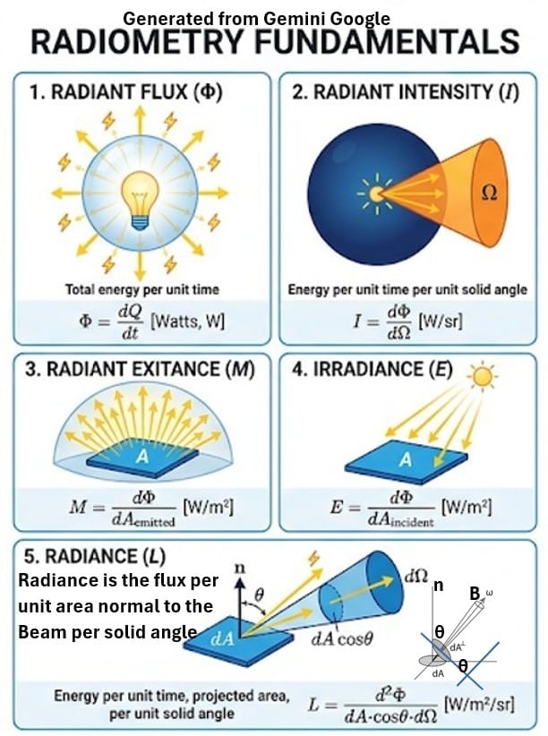
Summary
Spectral Radiance: Directional brightness from a specific patch at a specific angle (W / (m² · sr · m)).
Spectral Radiant Exitance (Emittance): Total light pouring out of a surface in all directions (W / m² / m).
Inverse-Square Calculation (I = P / 4π r²): How much total power is hitting a square meter out at distance r (Irradiance).
Appendix 8 – Understanding a Linear Spectral Curve vs a Linear/log2 Spectral Curve
Spectral radiant exitance (emittance or E) curves of bodies (sun and earth for our study) can be expressed traditionally with linear graphs of Emittance vs Wavelength (E vs λ like Graphs 1 and 2 below)
The primary disadvantage of the linear curves is that when comparing two bodies like the sun and the earth on the same plot, it is hard to make a visual assessment of the areas under the curves (as a direct indicator of total E).
You can use a little mathematical reconfiguration to come up with curves whose areas (representing total E) are much easier to “see” and compare. (like in Graph 3 below).
You just need to be careful to be clear of what you are looking at in each case, so below, for each graph type, we delineate their key features and how to use them.
Linear Spectral Curve
In graph 1, I show the spectral emittance (exitance) curve for the sun.
- Its shape is predicted by Planck’s Law equation and Weir’s Displacement Law.
- The peak of the curve indicates λmax
- and the shape shows you the distribution of the wavelength range with respect to emittance (exitance).
Graph_1: Linear Graph: Solar Radiation Spectrum for Sun at the Sun Surface
When you adjust it for E at the top of the earths atmosphere and plot it on the same graph as the earths spectrum you get Graph 2 below.
Graph_2 : Linear Graph: Solar Radiation Spectrum for Sun (at Earth TOA) and Earth
Graph 2 still gives us an idea of the peaks and spread of the curves but the areas underneath the curves (representing total E) are not easily visually comparable
Due to the large difference in wavelength ranges, the sun curve is a tall skinny curve and the earth curve is very flat and wide.
Primary Use: Best for analyzing absolute radiative magnitudes, physical emission peaks, and the true physical shape of the spectrum.
Key Features:
- True Distribution & Magnitude: Displays the actual, un-skewed distribution of emittance (E) across wavelengths, showing the massive scale difference between the Sun and Earth.
- Wien’s Law in Effect: The peak of each curve accurately points to λmax, clearly showing how the much hotter Sun emits at significantly shorter wavelengths than the cooler Earth.
- Area Limitation: While the mathematical area under each curve represents total energy, the extreme scale differences make visual comparison of these areas very difficult.
Linear vs Log2 Spectral Curve
Graph_3: Log-Wavelength Area-Preserving Plot
By multiplying E by λln(2) on the Y axis and plotting the log 2 of the wavelength on the X axis, we basically readjusted the widths and heights of the two curves and produced two bell shaped symmetrical shapes.
The amazing thing about this curve is, the areas under the curves still represent the total Energy and in this case, they are visually easy to compare.
Yes, the area looks bigger for the earth but that is because we are comparing the top of atmosphere incoming sun radiation with the earth surface radiation.
- The difference is explained by the point of measurement and also the presence of the earths atmosphere which contains warming agents like water and other molecules (greenhouse gases).
- Read all about the energy balance in the main text.
Primary Use: Best for visual comparison of total energy distribution and relative energy contributions between the Sun and Earth.
Key Features:
- Symmetrical Hills: Transformed into balanced, bell-like hills where total areas are easily distinguishable and comparable side-by-side.
- Loss of Spectral Intuition: Unlike Graph 1 and 2, the peaks do not correspond to λmax via Wien’s Law, and the curves do not reflect the true physical shape of the spectrum.
How Graph 3 Works (The Mechanics)
The X-Axis log2λ and “Octaves”
Plotting λ on a log base 2 scale means every octave (a doubling of wavelength, like 1 microns to 2 microns or 2 microns to 4 microns) takes up the exact same physical distance on the page.
This stretches the Sun’s short-wavelength curve (which is normally very compressed on a linear plot) and compresses the Earth’s long-wavelength curve (which is normally stretched out).
Picture: Log2λ X Axis Stretches Linear Sun Curve and Compresses Linear Earth Curve
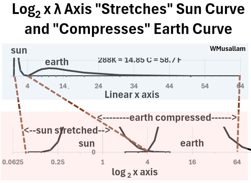
The Y-Axis Transformation Eλln(2)
Because the log scale distorts spatial widths, a standard Y-axis would visually misrepresent the energy.
Multiplying by λln(2) acts as a balancing weight:
- The λ factor cancels out the geometric stretching and compressing of the X-axis.
- The ln(2) factor accounts for the base-2 math.
- Result: This ensures the graph is area-preserving, meaning the visual area under each hill remains strictly proportional to the total physical energy emitted.
Return to “Earth and Sun Radiation Spectra Compared” Section
Appendix 9 – The Basic Physics of Climate Science
Here are some basic physics concepts needed to understand climate science.
Ideal Gas Law
One of the first things you learn in Chemistry class is the Idea Gas Law. It’s pretty accurate at low pressures and almost always indicative.
It will help you understand air behaviour when trying to understand the weather and climate.
In open space or the atmosphere, a gas occupies a defined regional space called a gas parcel or volume, and it exerts pressure against the surrounding air or any surface it touches.
9.1 PV = nRT
where (note that the units of measure for each variable MUST BE CONSISTENT; otherwise you will get garbage when you do the math) ,
- P = Pressure: The force per unit area exerted by colliding gas molecules against surrounding air or surfaces.
- SI Unit: Pascal = Pa; 1 Pa = 1 Newton per meter squared = 1 N/m²
- V = Volume: The three-dimensional space occupied by the gas sample.
- SI Unit: Cubic meter (m3)
- n (moles; Amount of a substance): The total count of gas particles.
- SI Unit: Mole (mol)
- R = Ideal Gas Constant: The fixed proportionality constant balancing the units in the equation
- SI Unit: 8.314 Joules per mole-Kelvin
- T = Absolute temperature: The measure of the average kinetic energy (speed) of the gas particles.
- SI Unit: Kelvin (K); T(0C) = T(K) – 273.15 and (T0F) = 1.8(T0C) + 32
In Climate Science , when analyzing air, the equation is often transformed into a more useful form:
Multiply both sides of equation 9.1 by the Molecular Weight of Air (MWa):
- MWa PV = MWa naRT
(MWa)(na)= Mass air = Ma so,
- MWa PV = MaRT
Divide both sides by V and MWa :
- P = (Ma/V)(R/MWa)(T)
Let the density of air be ρa = Ma/V and Specific R for air is Ra = R/MWa
9.2 P = ρ RaT
or
9.3 ρ = P/(RaT)
These equations are useful.
Equation 9.3 shows that the density is proportional to pressure and inversely proportional to temperature (which should be intuitive to you).
Archimedes’ Law
Any object partially or fully submerged in a fluid (liquid or gas) experiences an upward buoyant force equal to the weight of the fluid displaced
Let,
- mo = Mass of object or parcel
- mb = Mass of fluid displaced by object (parcel)
- g = the acceleration due to gravity = the rate at which a falling object speeds up near Earth’s surface (9.8 m/s²).
Fluid pressure exerts normal (perpendicular) forces on every surface of a submerged object or parcel—top, bottom, and all surrounding sides.
The horizontal forces cancel each other out, leaving only the net upward difference between the pressure on the bottom and the pressure on the top.
The net result of these vertical forces is called the buoyant force.
- Fb = mass x acceleration = upward buoyant force of displaced fluid = mbg = ρbVbg; remember that mass = density x volume
- Fo = downward force of gravity on an object = mog = ρoVog
We can do a force balance around an object or parcel (i.e. a solid object or a parcel of air)
9.4 Force Balance: Fnet = Fgravity – Fbuoyancy
Substitute for for F = mg:
Force Balance: (mscale)(g) = (mobject)(g) – (mfluid displaced)(g); where g = acceleration of gravity
The g’s cancel out so we get:
9.5 Force Balance: mscale = mobject – mfluid displaced
When you measure an object on a scale , the scale is actually calculating mass based on the force exerted by the object on the scale.
- If there is no (or negligible) buoyant force being produced, then the mass you read on a scale will equal the mass of the object.
- But, if you take a solid object and weigh it on a scale and then submerge it into water, its computed scale mass will change even though the mass of the object doesn’t change as expressed in equation 9.5.
The following example hopefully reinforces this point:
Picture: Archimedes’ Principle Example
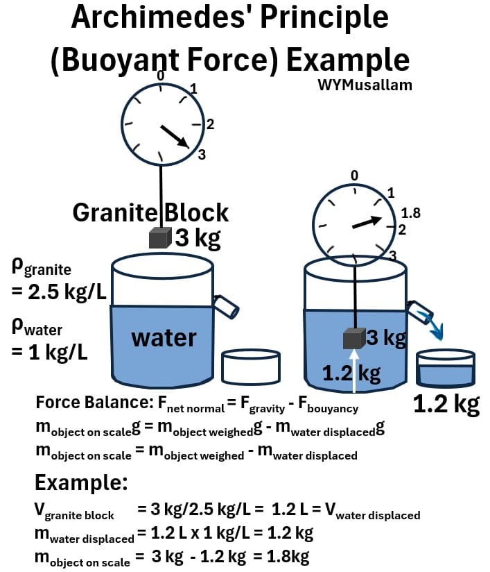
You can do the same force balance on a parcel of warm air (in surrounding cold air) or vice versa.
Force Balance on a Parcel of Air
A convection cell in climate science is an atmospheric circulation loop driven by temperature differences:
- warm, less dense air rises, cools at higher altitudes,
- sinks as it becomes denser,
- and flows back along the surface to complete the cycle.
Let’s apply the Ideal Gas Law and Archimedes’ Law to explain the rising and sinking of air.
Consider the picture below showing the movement of air in a convection cell.
Picture: Convection Cell Air Movement
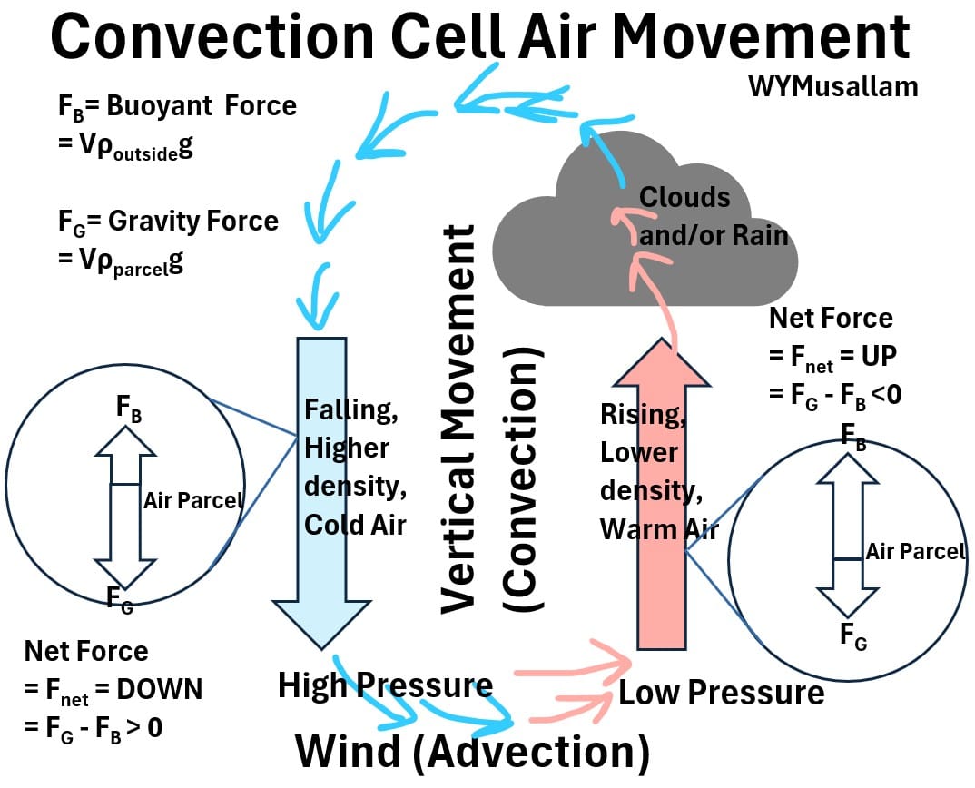
Let’s do a force balance around a parcel of air (see the schematic above).
Net Force = Downward Gravity Force – Upward Buoyancy Force
Recall 9.4: Force Balance: Fnet = Fgravity – Fbuoyancy
- If Fgravity > Fbuoyancy, then Fnet is positive and we have a net downward force (i.e. object or parcel moves down)
- If Fgravity < Fbuoyancy, then Fnet is negative and we have a net upward force (i.e. object or parcel moves up)
Substitute for Force = mass x acceleration
- Net Force = (mparcel air)(g) – (msurrounding air)(g)
We know that mass = density x volume so lets express mass this way:
- Net Force = ρparcel air Vg – ρsurrounding airVg
- Net Force = Vg(ρparcel air – ρρsurrounding air)
Substitute the Ideal Gas Law : (9.3) ρ = P/(RaT)
- Net Force = Vg ( P/(RaTparcel air) – P/(RaTsurrounding air) )
Factor out VgP/Ra :
- Net Force = VgP/Ra ( 1/(Tparcel air) – 1/(Tsurrounding air) )
Combine the two fractions into a single fraction:
9.6: Net Force = VgP/Ra ({Tsurrounding air – Tparcel air} / {Tparcel airTsurrounding air})
If the temperature of the air parcel is greater than the surrounding T
- Tsurrounding air < Tparcel air
- meaning the Net Force is negative, and because we defined it this way (Fnet = Fgravity – Fbuoyancy),
- the air parcel moves upwards (i.e. hot air rises)
If the temperature of the air parcel is less than the surrounding T
- Tsurrounding air > Tparcel air
- meaning the Net Force is positive, and because we defined it this way (Fnet = Fgravity – Fbuoyancy),
- the air parcel moves downwards (i.e. cold air descends)
Wind
We just described the net ascending or descending forces affecting the vertical movement of air (normally described as convection).
There is also a horizontal component that we called advection.
The air at the Earths surface (at the bottom of those columns of air in our picture above) will move from high pressure to low pressure areas (Pressure is just Force/Area….so higher Pressure means higher force per unit areas).
This is called wind.
Ideal Convection Cell Versus Reality
An idealized convection cell is represented as a simple, two-dimensional loop governed by thermal buoyancy.
- Warm, expanding air rises over a heated zone, while cool, dense air sinks over a colder region.
- Horizontal advection (surface wind) pushes air across the ground from the cold high-pressure region toward the warm low-pressure region,
- while an equal return wind flows horizontally aloft to complete a clean, closed rectangular circuit.
In reality, atmospheric motion is far more complex.
- Because horizontal temperature and pressure differences exist at every vertical position in the air column, horizontal winds occur continuously across all elevations—not just at the absolute top and bottom.
- Also, Earth’s rotation constantly deflects vertical moving currents (i.e. wind moving from equators to poles) sideways (called the Coriolis Effect which we’ll describe in the following appendix).
So it’s more complex but it is still true that the net bulk transport of air and heat in our atmosphere follow these convection loops (usually over 1000s of miles).
Mass Flux and Heat Flux Relationship
The sensible heat equation calculates how much thermal energy is absorbed, released, or transported when a material changes temperature without changing its phase.
When dealing with moving fluids (like air currents or water flows), we use the rate form to describe heat flux:
9.7 Q = m CpΔT ; Sensible Heat Transfer Equation
where
- Q (Heat Flux): The rate of thermal energy transferred (in Watts or Joules per second).
- m (Mass Flux): The amount of mass moving through a space per unit time (kg/s).
- Cp (Specific Heat Capacity): How much heat energy 1 kg of the substance can hold per 1C temperature change (units of J/kg/C).
- ΔT (Temperature Difference): For heat to flow ΔT has to be positive…i.e. High Temperature moving to Cold Temperature.
- Q = (kg/s)(J/kg/C)(C) = J/s
The “Bolt-On” Concept: Mass Carries the Heat
On its own, mass flux only measures how much matter is moving.
The heat flux (Q) is literally a thermal bolt-on to mass flux:
- Q (the Heat Flux) = m (the Mass Flux) x Cp ΔT (the “Bolt-On” Thermal Cargo)
- Mass flux acts as the conveyor belt.
- The term (Cp ΔT) is the thermal payload bolted onto that moving mass.
It’s the mass flows of the Earth’s atmosphere (winds and convection cells) and oceans that enable heat to transfer from hot regions to cold regions.
Appendix 10 – Earth’s Latitudinal Energy Balance (Wind and Waves)
We have said that the average earth temperature is 15 C or so, but obviously this is a composite representation (an average) of everywhere.
So it’s not necessarily accurate anywhere.
The graph below plots average annual global temperatures in each latitude.
Graph – Latitudinal Raw and Area Weighted Mean Annual Global Temperatures
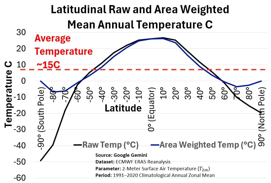
- While the raw data (black line) plunges into extreme sub-zero temperatures at the poles, the real-world geographic weight (blue line) collapses to zero at those edges.
- Because the massive, warm tropical center dominates 50% of the planet’s surface area, it anchors the global average (red line) firmly in the warm zone.
So temperatures on earth vary and this is caused by unequal distribution of solar radiation on the earths surface.
The Sun Heats The Earth Unequally
Consider the picture below.
Picture: The Sun Heats the Earth Unequally
It shows how Earth’s spherical shape creates the primary heat imbalance that drives global weather.
- Near the equator, sunlight strikes directly at a high angle, concentrating solar radiation into a small surface area for maximum energy density (Highest Energy/Area).
- Toward the poles, the shallow angle of incidence spreads that exact same beam of sunlight over a much larger surface area, resulting in a much lower energy density (Lowest Energy/Area).
This fundamental gap, a surplus of thermal energy at the tropics and a deficit at the poles, is what forces Earth’s weather and ocean currents to continuously move heat away from the equator.
Latitudinal Energy Balance
The graph below compares incoming solar energy against outgoing heat radiating back into space across all latitudes.
Latitude is the measurement of a location’s position north or south of the equator, expressed in degrees from 0° at the equator to 90° at the poles.
A way to remember this term is the shape of your mouth when you say it (as opposed to longitude).
Graph – Earth’s Latitudinal Energy Balance
- The Tropics (Surplus): Between about 35oS and 35oN, incoming sunlight (pink line) exceeds outgoing heat (green line).
- The equator absorbs far more energy than it releases, creating a massive heat surplus.
- The Poles (Deficit): Beyond 35-40 o in both directions, outgoing heat exceeds incoming sunlight.
- The polar regions radiate more energy into space than they receive from the sun, running a thermal deficit.
- The line intersection (at 35-40 o): These latitude lines are where incoming and outgoing energy temporarily balance out.
Without heat transport, the equator would continuously bake and the poles would freeze solid.
The double-headed blue arrow above represents atmospheric winds and ocean currents constantly carrying that surplus heat away from the equator and dumping it at the poles.
The next graph helps us understand even better the heat flow shown in the latitudinal heat balance picture by breaking down who moves the heat and where it goes.
Graph – Heat Transfer from the Tropics to the Poles
- Direction of Flow: Positive values (+Y) mean heat is moving North, and negative values (-Y) mean heat is moving South; showing that heat constantly flows away from the equator toward both poles.
- Peak Heat Flow: Total transport peaks around 35-40o latitude in both hemispheres, right at the boundary line where the equatorial heat surplus turns into a polar deficit.
- Ocean currents (blue line) carry a massive share of the heat in the tropics (10-20o).
- Atmospheric winds (red line) take over in the mid-to-high latitudes (30-80o), carrying the vast majority of the heat the rest of the way to the poles.
The below combined view links the energy graph directly onto Earth’s geography.
Graph – Latitudinal Energy Balance Mapped to Earth’s Latitudes
- Alignment: The graph is turned on its side to map latitude for latitude onto the globe—showing the tropical energy surplus around 0o and the polar energy deficits from 60-90o North and South.
- The Global Engine: The arrows on the globe summarize the end result: planetary wind circulation and ocean currents act together as a massive transport system, driving net heat away from the tropics to balance out the cold poles.
Before we describe currents and winds in any detail we first need to describe the Coriolis Effect.
Coriolis Effect
Analogy Set Up
Consider the picture below as you read through the spinning device analogy.
Picture: Coriolis Effect: Spinning Device Modelling
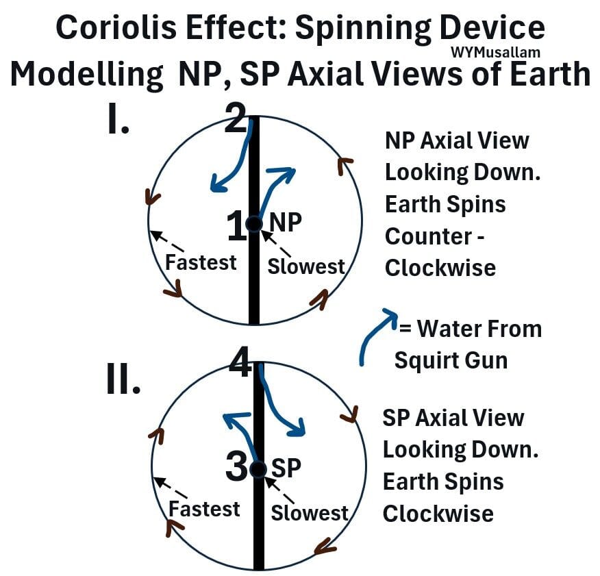
Diagram Explanation
The circles represent top-down views along Earth’s rotational axis:
- Circle I (North Pole View): Represents looking down at the North Pole from space. From this angle, Earth rotates counter-clockwise.
- Circle II (South Pole View): Represents looking down at the South Pole. From this angle, Earth rotates clockwise.
- Center (1 & 3): The geographical pole—the axis of rotation where the surface rotational speed is zero (slowest).
- Outer Rim (2 & 4): The Equator, where the surface moves at maximum speed (fastest).
- Black Line: A straight reference line across the surface, like a circle diameter line or a straight plank mounted on a rotating rig.
Set Up: The Spinning Earth Model
The model I describe here is based on this great video: The Coriolis Effect Explained – DeverScience
We want to build a model that will mimic the Earth’s motion describe in the circle diagram above.
- Install a straight balanced plank on a central spinning wheel (i.e. a turntable or an actual wheel installed sideways on its spinning axis).
- the plank will serve as a straight reference line.
- Mount 2 squirt guns on the plank.
- One at the center (position 1 or 3 in the circle diagram), pointed outward along the plank toward the rim.
- One at the outer edge (2 or 4), pointed inward along the plank toward the center.
Spin The Model (Refer to the Circle Diagrams Above)
If we spin the plank counterclockwise, we mimic Earth’s rotation from a North Pole reference point and if we spin the plank clockwise we mimic Earth’s rotation from the South Pole.
Once a stream of water leaves the squirt gun nozzle, it travels in a straight line through the air relative to the room (due to inertia).
- However, it retains whatever sideways speed it had at the moment it was fired.
- Because different points on the spinning plank move at different sideways speeds, the plank moves out from underneath the stream.
Scenario 1: Counter-Clockwise Spin (North Pole View)
Water Stream Goes from Center to Rim (1 → 2)
- The water lags behind the plank and curves to the right of its path
- because the center (1) has zero sideways speed.
- As the water flies toward the rim, the outer plank (2) is moving fast to the left.
- The water lacks the sideways speed to keep up, so the plank sweeps away from under it.
Water Stream Goes from Rim to Center (2 → 1)
- The water leads ahead of the plank and curves to its right
- because the rim (2) is moving fast to the left.
- The water leaves the gun carrying that high leftward speed.
- As it travels inward toward the slow-moving center (1), it moves sideways faster than the plank underneath it, cutting ahead of the line.
Scenario 2: Clockwise Spin (South Pole View)
Water Stream Goes from Center to Rim (3 → 4)
- The water lags behind and curves to the left of its path.
- because fired from the slow center (3), the water has minimal sideways motion.
- The fast-moving rim (4) spins rightward away from the stream, leaving the water trailing behind.
Water Stream Goes from Rim to Center (4 → 3)
- The water leads ahead and curves to its left
- because fired from the fast rightward-moving rim (4), the stream carries that momentum inward.
- It outpaces the slower center plank (3), drifting ahead of the reference line to the left.
Coriolis Affects The Wind and Ocean Directional Movement
The Coriolis effect is a frame-of-reference effect resulting from observing motion from inside a rotating system.
It acts directly on anything moving across Earth’s surface—water, air, aircraft, rockets, etc.
It shapes global wind patterns, rotates hurricane systems, alters ocean currents, and affects long-range trajectories.
Because the planet rotates beneath moving paths, every unanchored mass curves relative to the ground
- to the right (looking in the direction of movement) in the Northern Hemisphere and
- to the left (looking in the direction of movement) in the Southern Hemisphere.
Picture: Coriolis Effect: Air and Water Movement Deflection on Earth
The Coriolis effect first deflects global winds as they blow across pressure gradients in the atmosphere.
When those turned winds push against the ocean, direct Coriolis forces act on the moving water itself, deflecting its path a second time.
- This continuous deflection forces ocean currents into giant circular loops called gyres (pronounced jyres), which steer warm and cold water across the globe.
- At the same time, as surface water moves, it pulls deeper layers of water along with it.
- Because each deeper layer gets turned even further by Earth’s spin, it creates a twisting downward pattern known as the Ekman spiral.
For a nice lecture on the above see: Lecture #42 Climate Change – Surface Currents and Upwelling – Colin Price
The map below shows the major ocean gyres. These handle the oceanic side of global heat transport.
Picture: Gyres – Earth’s Rotating Ocean Currents (Surface Waters)
- Warm Currents (Red Arrows): Move heated tropical water poleward along western ocean margins (e.g., the Gulf Stream and Kuroshio).
- Cold Currents (Blue Arrows): Return chilled polar water back toward the equator along eastern ocean margins (e.g., the California and Canary currents).
- The Giant Loop: These rotating gyres act as massive planetary conveyor belts, physically sweeping surplus energy out of the tropics and pushing it toward the cold poles.
While surface gyres move top-layer water, thermohaline circulation (the Great Ocean Conveyor Belt) takes heat transport into three dimensions, driven by temperature and salinity density differences.
- Ocean gyres are shallow surface currents confined to the top 1,000 meters where wind friction reaches.
- In contrast, the Great Ocean Conveyor Belt plunges 2,000 to 4,000+ meters down, circulating water along the deep (abyssal) ocean floor.
Consider the drawing below.
Picture – Thermohaline Circulation – Great Ocean Conveyor Belt
- What is AMOC? The Atlantic Meridional Overturning Current is the Atlantic “engine” of this global belt.
- AMOC acts as a massive oceanic heat pump: pulling warm tropical water north along the surface, dumping heat into the northern atmosphere, sinking as cold, salty water near Greenland, and pushing deep water back south.
- Climate scientists warn that if AMOC collapses, Northern Europe cools dramatically and global weather shifts instantly.
- The 1,000-Year Loop: Because the deep ocean moves so slowly, it takes a single parcel of water roughly 1,000 years to complete one full loop around the world.
- Surface Heat Transport (Red Lines): Shallow warm currents carry tropical energy north into the Atlantic and Pacific.
- Deep Return Circuit (Blue Lines): Chilled, dense water sinks into the deep ocean and flows south across the planet’s floor, linking all major oceans into one connected climate regulator.
The General Circulation of the Atmosphere
General Circulation of the Atmosphere is the large-scale, continuous movement of air around the Earth that distributes thermal energy from the equator to the poles.
A fundamental mechanism in the general circulation of the atmosphere is the convection cell which we studied in the physics section (Appendix 9)
Picture – Convection Cell Air Movement

This diagram illustrates the fundamental mechanics of a basic convection cell and shows how surface pressure differences are created (we reviewed this in Appendix 9 as well):
- Low Pressure Zone: Warm, low-density air rises as buoyant force overcomes gravity.
- As the air ascends, it cools and expands, forming clouds and precipitation, while leaving behind a region of lower surface pressure.
- High Pressure Zone: Cold, high-density air sinks as gravity pulls it back down toward the ground.
- This descending air presses against Earth’s surface, creating a high-pressure region.
- Surface Wind (Advection): To replace the rising air, surface air flows horizontally from the high-pressure area toward the low-pressure area.
- The Hadley, Ferrel, and Polar cells in global atmospheric circulation (see picture below) each function as an individual loop built on this exact convection mechanism.
The picture below illustrates Earth’s global atmospheric circulation model, depicting the three major circulation cells, surface wind patterns, and pressure belts in each hemisphere.
Picture – Atmospheric Circulation (Convection Cells and Winds)
Air naturally moves from high-pressure belts to low-pressure belts, but Earth’s rotation prevents it from traveling in a straight line.
The Coriolis effect, as we’ve demonstrated, deflects this moving air to its right in the Northern Hemisphere and to its left in the Southern Hemisphere.
As air flows north and south between the pressure zones, this lateral deflection bends the surface winds into the distinct east-west patterns shown in the picture.
Atmospheric Convection Cells
- Hadley Cell: 0° (Equator) to 30° N/S.
- Ferrel Cell (Mid-latitude): 30° N/S to 60° N/S.
- Polar Cell: 60° N/S to 90° N/S (Poles).
Surface Wind Patterns
These are named relative to their starting position.
- Trade Winds (Northeasterly/Southeasterly):Blow east-to-west from 30° N/S toward the Equator.
- Westerlies: Blow west-to-east between 30° N/S and 60° N/S.
- Polar Easterlies: Blow east-to-west from 90° N/S toward 60° N/S.
Pressure Zones
- Low Pressure (L.P.): Located at the Equator (Doldrums / ITCZ) and at 60° N/S.
- High Pressure (H.P.): Located at 30° N/S (Horse Latitudes) and at the Poles (90° N/S).
In the drawing above , you will note pairs of black arrows between the Hadley, Ferrel ,and Polar cells which point vertically away or towards earth (Up/Down).
- These are the air upflow and downflow sections of the convection cell.
Because air moves up or down in these zones instead of across the ground, surface winds drop to almost zero.
That lack of wind is how the Doldrums (at the equator) and the Horse Latitudes (at 30°) got their names.
Doldrums
- Derived from an old English word meaning “dull” or “sluggish.”
- Because air rises at the equator rather than blowing horizontally, winds are extremely weak.
- Sailing ships often got trapped here for weeks in hot, motionless weather, leaving crews stuck in a state of stagnation and low spirits.
Horse Latitudes
- Named during the era of Spanish sailing ships traveling to the Americas.
- Sinking air in these high-pressure belts creates calm, windless conditions.
- When ships became stalled for long periods and ran short on drinking water, sailors were forced to throw dead or dying horses overboard to conserve water and lighten the load
Return to “Earth’s Latitudinal Energy Balance (Wind and Waves)” Section